Unstructured data refers to data that is not organized in any way, such as:
images,
texts,
sounds,
videos.
Regardless of the type, we process everything into tensors (multi-dimensional arrays). This may lead to the desire to use ML models and neural networks for analyzing unstructured data.
Let’s start with images.
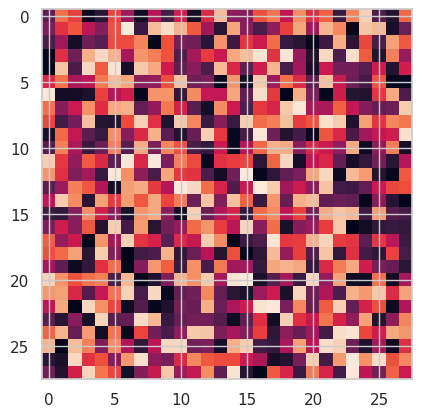
Create a 2-dim picture with random pixels.
import numpy as npimport seaborn as snsimport matplotlib.pyplot as pltsns.set(style="whitegrid", palette="husl")# 2-dim picture 28 x 28 pixelpicture_2d = np.random.uniform(size=(28,28))picture_2d[0:5,0:5]
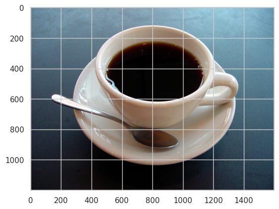
Creating batch size - an additional dimension (for other images)
batch = img_tensor.unsqueeze(0)batch.shape
torch.Size([1, 3, 224, 224])
Load alexnet model
from torchvision import models
model = models.alexnet(pretrained=True)
/opt/conda/lib/python3.11/site-packages/torchvision/models/_utils.py:208: UserWarning: The parameter 'pretrained' is deprecated since 0.13 and may be removed in the future, please use 'weights' instead.
  warnings.warn(
/opt/conda/lib/python3.11/site-packages/torchvision/models/_utils.py:223: UserWarning: Arguments other than a weight enum or `None` for 'weights' are deprecated since 0.13 and may be removed in the future. The current behavior is equivalent to passing `weights=AlexNet_Weights.IMAGENET1K_V1`. You can also use `weights=AlexNet_Weights.DEFAULT` to get the most up-to-date weights.
  warnings.warn(msg)
Downloading: "https://download.pytorch.org/models/alexnet-owt-7be5be79.pth" to /home/jovyan/.cache/torch/hub/checkpoints/alexnet-owt-7be5be79.pth
100%|██████████| 233M/233M [00:04<00:00, 50.2MB/s]
Let’s write universal code that you can run on both GPU and CPU
# Define the losscriterion = nn.NLLLoss()# Define the optimizeroptimizer = optim.Adam(model.parameters(), lr =0.002)
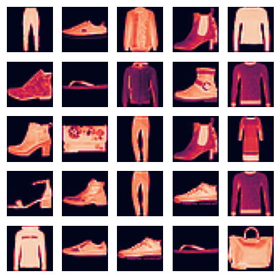
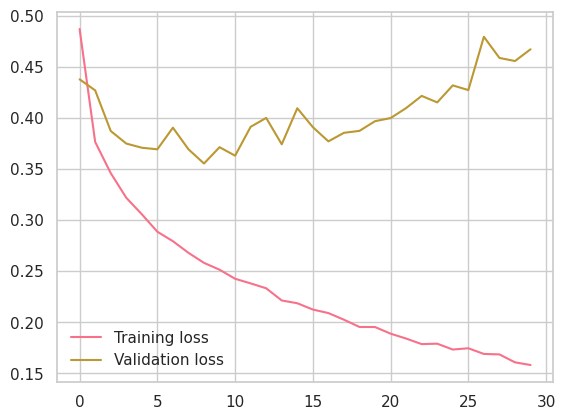
# Define the epochsepochs =30train_losses, test_losses = [], []for e inrange(epochs): running_loss =0for images, labels in trainloader:# Flatten Fashion-MNIST images into a 784 long vector images = images.view(images.shape[0], -1)# Training pass optimizer.zero_grad() output = model.forward(images) loss = criterion(output, labels) loss.backward() optimizer.step() running_loss += loss.item()else: test_loss =0 accuracy =0# Turn off gradients for validation, saves memory and computationwith torch.no_grad():# Set the model to evaluation mode model.eval()# Validation passfor images, labels in testloader: images = images.view(images.shape[0], -1) log_ps = model(images) test_loss += criterion(log_ps, labels) ps = torch.exp(log_ps) top_p, top_class = ps.topk(1, dim =1) equals = top_class == labels.view(*top_class.shape) accuracy += torch.mean(equals.type(torch.FloatTensor)) model.train() train_losses.append(running_loss/len(trainloader)) test_losses.append(test_loss/len(testloader))print("Epoch: {}/{}..".format(e+1, epochs),"Training loss: {:.3f}..".format(running_loss/len(trainloader)),"Test loss: {:.3f}..".format(test_loss/len(testloader)),"Test Accuracy: {:.3f}".format(accuracy/len(testloader)))
Epoch: 1/30.. Training loss: 0.487.. Test loss: 0.438.. Test Accuracy: 0.837
Epoch: 2/30.. Training loss: 0.377.. Test loss: 0.427.. Test Accuracy: 0.845
Epoch: 3/30.. Training loss: 0.346.. Test loss: 0.387.. Test Accuracy: 0.864
Epoch: 4/30.. Training loss: 0.322.. Test loss: 0.375.. Test Accuracy: 0.865
Epoch: 5/30.. Training loss: 0.306.. Test loss: 0.371.. Test Accuracy: 0.871
Epoch: 6/30.. Training loss: 0.289.. Test loss: 0.369.. Test Accuracy: 0.865
Epoch: 7/30.. Training loss: 0.279.. Test loss: 0.390.. Test Accuracy: 0.865
Epoch: 8/30.. Training loss: 0.268.. Test loss: 0.369.. Test Accuracy: 0.872
Epoch: 9/30.. Training loss: 0.258.. Test loss: 0.355.. Test Accuracy: 0.878
Epoch: 10/30.. Training loss: 0.251.. Test loss: 0.371.. Test Accuracy: 0.874
Epoch: 11/30.. Training loss: 0.243.. Test loss: 0.363.. Test Accuracy: 0.879
Epoch: 12/30.. Training loss: 0.238.. Test loss: 0.391.. Test Accuracy: 0.870
Epoch: 13/30.. Training loss: 0.233.. Test loss: 0.400.. Test Accuracy: 0.875
Epoch: 14/30.. Training loss: 0.221.. Test loss: 0.374.. Test Accuracy: 0.883
Epoch: 15/30.. Training loss: 0.219.. Test loss: 0.409.. Test Accuracy: 0.875
Epoch: 16/30.. Training loss: 0.212.. Test loss: 0.391.. Test Accuracy: 0.880
Epoch: 17/30.. Training loss: 0.209.. Test loss: 0.377.. Test Accuracy: 0.882
Epoch: 18/30.. Training loss: 0.203.. Test loss: 0.385.. Test Accuracy: 0.884
Epoch: 19/30.. Training loss: 0.195.. Test loss: 0.387.. Test Accuracy: 0.883
Epoch: 20/30.. Training loss: 0.195.. Test loss: 0.397.. Test Accuracy: 0.883
Epoch: 21/30.. Training loss: 0.189.. Test loss: 0.400.. Test Accuracy: 0.883
Epoch: 22/30.. Training loss: 0.184.. Test loss: 0.410.. Test Accuracy: 0.882
Epoch: 23/30.. Training loss: 0.179.. Test loss: 0.422.. Test Accuracy: 0.880
Epoch: 24/30.. Training loss: 0.179.. Test loss: 0.415.. Test Accuracy: 0.880
Epoch: 25/30.. Training loss: 0.173.. Test loss: 0.432.. Test Accuracy: 0.876
Epoch: 26/30.. Training loss: 0.175.. Test loss: 0.427.. Test Accuracy: 0.882
Epoch: 27/30.. Training loss: 0.169.. Test loss: 0.479.. Test Accuracy: 0.876
Epoch: 28/30.. Training loss: 0.169.. Test loss: 0.459.. Test Accuracy: 0.873
Epoch: 29/30.. Training loss: 0.161.. Test loss: 0.456.. Test Accuracy: 0.879
Epoch: 30/30.. Training loss: 0.158.. Test loss: 0.467.. Test Accuracy: 0.879
My model:

 Sequential(
  (0): Linear(in_features=784, out_features=128, bias=True)
  (1): ReLU()
  (2): Linear(in_features=128, out_features=10, bias=True)
  (3): LogSoftmax(dim=1)
)

The state dict keys:

 odict_keys(['0.weight', '0.bias', '2.weight', '2.bias'])
Text data and BoW model
import pandas as pddf_train = pd.read_csv("train.csv")df_train = df_train.drop("index", axis=1)print(df_train.head())print(np.bincount(df_train["label"]))
                                                text  label
0  When we started watching this series on cable,...      1
1  Steve Biko was a black activist who tried to r...      1
2  My short comment for this flick is go pick it ...      1
3  As a serious horror fan, I get that certain ma...      0
4  Robert Cummings, Laraine Day and Jean Muir sta...      1
[17452 17548]
# BoW model from sklearn.feature_extraction.text import CountVectorizercv = CountVectorizer(lowercase=True, max_features=10_000, stop_words="english")cv.fit(df_train["text"])
In a Jupyter environment, please rerun this cell to show the HTML representation or trust the notebook. On GitHub, the HTML representation is unable to render, please try loading this page with nbviewer.org.