---
title: "Lecture 2 — Batch vs Stream. Lambda and Kappa Architectures"
subtitle: "Real-Time Data Analytics"
description: "Batch vs stream processing, Lambda and Kappa architectures, event time, watermarking and time windows."
format:
html:
code-fold: true
code-tools: true
code-summary: "Show code"
toc: true
toc-depth: 3
toc-title: "Contents"
number-sections: true
smooth-scroll: true
theme:
light: flatly
highlight-style: github
fig-align: center
fig-cap-location: bottom
jupyter: python3
---
::: {.callout-note appearance="minimal"}
## Duration: 1.5h
**Goal:** Understand the differences between batch and stream processing, learn about Lambda and Kappa architectures, and key concepts: event time, processing time, time windows.
:::
---
## Batch vs Stream — two approaches to the same data
In the previous lecture we established that data **always** originates as a stream of events. Batch processing is just a simplification — we collect the stream into a file and analyze it with a delay.
Let's compare both approaches on the same business problem: **monitoring transactions in an online store**.
::: {.panel-tabset}
### {{< fa database >}} Batch approach
```{python}
import pandas as pd
import numpy as np
from datetime import datetime, timedelta

np.random.seed(42)

# Data collected throughout the day — analyzed the next morning
transactions = pd.DataFrame({
    'time': [datetime(2026, 3, 12, h, m)
             for h in range(9, 18)
             for m in np.random.choice(range(60), 20)],
    'amount': np.random.uniform(20, 3000, 180).round(2),
    'customer_id': np.random.randint(1000, 9999, 180)
})

# Daily report — we see it THE NEXT DAY
report = transactions.groupby(transactions['time'].dt.hour).agg(
    count=('amount', 'count'),
    total=('amount', 'sum'),
    average=('amount', 'mean')
).round(2)

print("Daily report (generated the next morning):")
print(report.head())
```
### {{< fa bolt >}} Stream approach
```{python}
import time

# Simulation: each transaction analyzed the moment it appears
window_5min = []
alert_threshold = 5000  # alert if window sum > 5000 PLN

for i in range(10):
    tx = {
        'time': datetime.now().strftime('%H:%M:%S'),
        'amount': round(np.random.uniform(20, 3000), 2),
        'customer': np.random.randint(1000, 9999)
    }
    window_5min.append(tx['amount'])
    window_sum = sum(window_5min)

    status = ""
    if window_sum > alert_threshold:
        status = " << ALERT: high activity!"
        window_5min = []  # reset window

    print(f"[{tx['time']}] Customer {tx['customer']}: {tx['amount']:>8.2f} PLN | Window sum: {window_sum:>9.2f}{status}")
    time.sleep(0.2)
```
:::
::: {.callout-important}
## The fundamental difference
In batch mode we learn about a problem **the next day**. In stream mode — **immediately**.
:::
---
## Lambda Architecture
In practice, companies need **both** approaches simultaneously. Lambda architecture, proposed by Nathan Marz, combines batch and stream processing in a single system.
### Three layers of Lambda
:::: {.columns}
::: {.column width="33%"}
::: {.callout-note appearance="simple"}
## {{< fa database >}} Batch layer
**Batch Layer** — processes the complete dataset at regular intervals. Produces accurate results, but with a delay.
*Tools:* Spark (batch), Hadoop
:::
:::
::: {.column width="33%"}
::: {.callout-warning appearance="simple"}
## {{< fa bolt >}} Speed layer
**Speed Layer** — processes streaming data in real time. Produces approximate results, but immediately.
*Tools:* Spark Streaming, Kafka Streams
:::
:::
::: {.column width="33%"}
::: {.callout-tip appearance="simple"}
## {{< fa server >}} Serving layer
**Serving Layer** — merges results from both layers and exposes them to end users.
*Tools:* databases, APIs, dashboards
:::
:::
::::
```{mermaid}
%%| fig-cap: "Lambda Architecture"
flowchart TD
    SRC["Data source\n(stream of events)"] --> BATCH["Batch Layer\nComplete data\nHigh latency"]
    SRC --> SPEED["Speed Layer\nLatest data\nLow latency"]
    BATCH --> SERVE["Serving Layer\nDashboard / API"]
    SPEED --> SERVE

    style BATCH fill:#2196F3,color:#fff
    style SPEED fill:#F44336,color:#fff
    style SERVE fill:#4CAF50,color:#fff
```
::: {.callout-tip collapse="true"}
## {{< fa building-columns >}} Business example: Bank analyzing card transactions
- **Batch layer:** every night recalculates historical customer behavior patterns, trains fraud detection models.
- **Speed layer:** in real time compares each transaction against patterns and blocks suspicious operations.
- **Serving layer:** analyst dashboard + mobile app API.
:::
### Lambda advantages and disadvantages
**Advantage:** completeness — the batch layer corrects speed layer errors.
::: {.callout-caution}
## Lambda's main drawback
You maintain **two separate processing pipelines** — two codebases, two test suites, two environments. This is expensive and error-prone.
:::
---
## Kappa Architecture
Jay Kreps (creator of Apache Kafka) proposed a simplification: **what if we only needed the streaming layer?**
Kappa architecture is Lambda without the batch layer. The entire data flow is based on a stream of events. If historical data needs to be reprocessed — we replay the stream from the beginning.
```{mermaid}
%%| fig-cap: "Kappa Architecture — a simplification of Lambda"
flowchart TD
    SRC["Data source\n(stream of events)"] --> STREAM["Stream Layer\nOne codebase, one pipeline"]
    STREAM --> SERVE["Serving Layer\nDashboard / API"]
    STREAM -.->|replay| SRC

    style STREAM fill:#FF9800,color:#fff
    style SERVE fill:#4CAF50,color:#fff
```
### Lambda vs Kappa — when to use which?
| Feature | {{< fa layer-group >}} Lambda | {{< fa arrows-turn-right >}} Kappa |
|-------|--------|-------|
| Complexity | High (two pipelines) | Low (one pipeline) |
| Accuracy | Batch corrects stream | Depends on streaming quality |
| Historical reprocessing | Natural (batch) | Stream replay |
| When to use | When batch and stream have different logic | When one logic is sufficient |
| Example | Bank (nightly retraining + RT scoring) | E-commerce (personalization) |
: Lambda vs Kappa {.striped .hover}
---
## Time in stream processing
In batch processing, time is not a problem — we analyze historical data whenever we want. In stream processing, time becomes a **key dimension of analysis**.
### Two kinds of time
:::: {.columns}
::: {.column width="50%"}
::: {.callout-note appearance="simple"}
## {{< fa calendar-day >}} Event time
The moment the event **actually occurred**.
*E.g., a customer clicked "Buy" at 14:23:45.*
:::
:::
::: {.column width="50%"}
::: {.callout-warning appearance="simple"}
## {{< fa server >}} Processing time
The moment the system **received and processed** the event.
*E.g., the Kafka system received the event at 14:23:47.*
:::
:::
::::
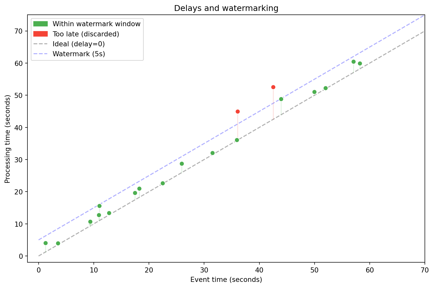
In an ideal world both times would be identical. In practice there is always a **delay** (latency) — caused by network, buffering, device failure.
```{python}
# Simulation: events arrive with random delay
import random

events = []
for i in range(8):
    event_time = datetime(2026, 3, 12, 14, 23, i * 2)  # every 2 seconds
    delay = random.uniform(0.1, 5.0)  # delay 0.1–5s
    processing_time = event_time + timedelta(seconds=delay)
    events.append({
        'event_time': event_time.strftime('%H:%M:%S'),
        'processing_time': processing_time.strftime('%H:%M:%S.') + f'{int(delay*100):02d}',
        'delay': f'{delay:.1f}s'
    })

df = pd.DataFrame(events)
print(df.to_string(index=False))
```
```{python}
#| label: fig-event-vs-processing
#| fig-cap: "Event time vs processing time — delays in streaming systems"
import matplotlib.pyplot as plt
import matplotlib.patches as mpatches

np.random.seed(42)
n = 20
evt = np.sort(np.random.uniform(0, 60, n))
delays = np.random.exponential(3, n)
proc = evt + delays
watermark = 5

fig, ax = plt.subplots(figsize=(9, 6))
ax.plot([0, 70], [0, 70], 'k--', alpha=0.3, label='Ideal (delay=0)')
ax.plot([0, 70], [watermark, 70+watermark], 'b--', alpha=0.3, label=f'Watermark ({watermark}s)')

for i in range(n):
    in_wm = proc[i] <= evt[i] + watermark + 1
    color = '#4CAF50' if in_wm else '#F44336'
    ax.scatter(evt[i], proc[i], c=color, s=50, zorder=5, edgecolors='white')
    ax.plot([evt[i], evt[i]], [evt[i], proc[i]], color=color, alpha=0.2, linewidth=1)

gp = mpatches.Patch(color='#4CAF50', label='Within watermark window')
rp = mpatches.Patch(color='#F44336', label='Too late (discarded)')
ax.legend(handles=[gp, rp, ax.lines[0], ax.lines[1]], loc='upper left')
ax.set_xlabel('Event time (seconds)')
ax.set_ylabel('Processing time (seconds)')
ax.set_title('Delays and watermarking')
ax.set_xlim(-2, 70)
ax.set_ylim(-2, 75)
plt.tight_layout()
plt.show()
```
::: {.callout-tip collapse="true"}
## {{< fa car >}} Analogy: GPS in a tunnel
Imagine tracking a car by GPS. The vehicle enters a tunnel — for 30 seconds there is no signal. After exiting, the device sends 30 readings at once. The system needs to know that these events belong to the **past**, not the present.
:::
Late events can be handled in two ways:
- **Ignoring** — discard events that arrived too late (risk of data loss).
- **Watermarking** — define a "watermark" — the maximum allowed delay. Events within the watermark window are included; the rest are discarded.
---
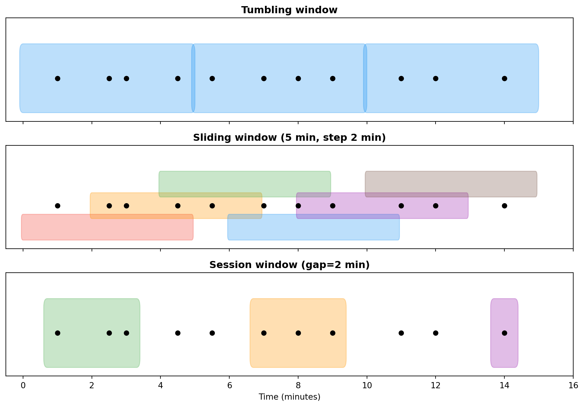
## Time windows
In stream processing we can't analyze "all data" — the stream is infinite. Instead, we group events into **time windows** of finite length.
::: {.panel-tabset}
### Tumbling
Fixed length, no overlap. Each event belongs to **exactly one** window.
*Example:* sum of transactions every 5 minutes.
```{python}
# Simulation of a 5-minute tumbling window
np.random.seed(42)

events = pd.DataFrame({
    'time': pd.date_range('2026-03-12 14:00', periods=30, freq='30s'),
    'amount': np.random.uniform(10, 500, 30).round(2)
})

# Tumbling window: grouping every 5 minutes
events['window'] = events['time'].dt.floor('5min')
result = events.groupby('window')['amount'].agg(['sum', 'count']).round(2)
result.columns = ['total', 'count']
print("Tumbling window (5 min):")
print(result)
```
### Sliding
Fixed length, but the window slides by a given interval — events can belong to **multiple windows**.
*Example:* average over the last 10 minutes, updated every 2 minutes. Useful for detecting trends.
### Hopping
Similar to sliding, but with overlap at a specific step. Used for data smoothing.
### Session
Dynamic length — the window lasts as long as events keep arriving. Closes after a specified period of inactivity (**gap**).
*Example:* user session on a website. The session lasts while the user clicks. Closes after 15 minutes of inactivity.
:::
### Window comparison
| Window type | Length | Overlap | Use case |
|----------|---------|:----------:|-------------|
| Tumbling | Fixed | {{< fa xmark >}} | Periodic reports |
| Sliding | Fixed | {{< fa check >}} | Trend detection |
| Hopping | Fixed | Partial | Data smoothing |
| Session | Dynamic | {{< fa xmark >}} | User session analysis |
: Time window types {.striped .hover}
```{python}
#| label: fig-window-types
#| fig-cap: "Time window types — visualization"
import matplotlib.pyplot as plt
import matplotlib.patches as mpatches

fig, axes = plt.subplots(3, 1, figsize=(10, 7), sharex=True)

events_x = [1, 2.5, 3, 4.5, 5.5, 7, 8, 9, 11, 12, 14]

# Tumbling
ax = axes[0]
ax.set_title('Tumbling window', fontweight='bold')
for start in range(0, 15, 5):
    rect = mpatches.FancyBboxPatch((start, 0.2), 4.9, 0.6, boxstyle="round,pad=0.1",
        facecolor='#2196F3', alpha=0.3, edgecolor='#2196F3')
    ax.add_patch(rect)
ax.scatter(events_x, [0.5]*len(events_x), c='black', s=30, zorder=5)
ax.set_ylim(0, 1.2)
ax.set_yticks([])

# Sliding
ax = axes[1]
ax.set_title('Sliding window (5 min, step 2 min)', fontweight='bold')
colors = ['#F44336', '#FF9800', '#4CAF50', '#2196F3', '#9C27B0', '#795548', '#607D8B']
for i, start in enumerate(range(0, 12, 2)):
    y_offset = 0.15 + (i % 3) * 0.25
    rect = mpatches.FancyBboxPatch((start, y_offset), 4.9, 0.2, boxstyle="round,pad=0.05",
        facecolor=colors[i % len(colors)], alpha=0.3, edgecolor=colors[i % len(colors)])
    ax.add_patch(rect)
ax.scatter(events_x, [0.5]*len(events_x), c='black', s=30, zorder=5)
ax.set_ylim(0, 1.2)
ax.set_yticks([])

# Session
ax = axes[2]
ax.set_title('Session window (gap=2 min)', fontweight='bold')
session_events = [[1, 2.5, 3], [7, 8, 9], [14]]
sess_colors = ['#4CAF50', '#FF9800', '#9C27B0']
for j, (sess, col) in enumerate(zip(session_events, sess_colors)):
    start = min(sess) - 0.3
    end = max(sess) + 0.3
    rect = mpatches.FancyBboxPatch((start, 0.2), end-start, 0.6, boxstyle="round,pad=0.1",
        facecolor=col, alpha=0.3, edgecolor=col)
    ax.add_patch(rect)
ax.scatter(events_x, [0.5]*len(events_x), c='black', s=30, zorder=5)
ax.set_ylim(0, 1.2)
ax.set_yticks([])
ax.set_xlabel('Time (minutes)')
ax.set_xlim(-0.5, 16)

plt.tight_layout()
plt.show()
```
```{python}
# Comparison: tumbling vs sliding window on the same data
print("=== Tumbling (5 min) ===")
tumbling = events.groupby(events['time'].dt.floor('5min'))['amount'].sum().round(2)
print(tumbling)

print("\n=== Sliding (5 min window, 1 min step) ===")
for start_min in range(0, 15, 1):
    start = pd.Timestamp('2026-03-12 14:00') + pd.Timedelta(minutes=start_min)
    end = start + pd.Timedelta(minutes=5)
    mask = (events['time'] >= start) & (events['time'] < end)
    total = events.loc[mask, 'amount'].sum()
    if total > 0:
        print(f"  [{start.strftime('%H:%M')}–{end.strftime('%H:%M')}) total = {total:.2f}")
```
---
## Summary
In this lecture we learned about two key architectures (Lambda and Kappa) and the fundamental concepts of stream processing: event time, processing time, watermarking and time windows. These concepts will accompany us in the labs when working with Apache Kafka and Spark Structured Streaming.
::: {.callout-note appearance="simple"}
## {{< fa forward >}} Next lecture
Machine learning in batch and incremental (online learning) modes, Stochastic Gradient Descent, anomaly detection.
:::
::: {.callout-tip appearance="simple"}
## {{< fa brain >}} Food for thought
Your client wants a sales dashboard updated every 30 seconds. What architecture (Lambda/Kappa) would you propose? What type of time window would you use?
:::