---
title: "Lecture 3 — Machine Learning: batch vs online"
subtitle: "Real-Time Data Analytics"
description: "Batch vs incremental learning, SGD, concept drift, anomaly detection and model explainability."
format:
html:
code-fold: true
code-tools: true
code-summary: "Show code"
toc: true
toc-depth: 3
toc-title: "Contents"
number-sections: true
smooth-scroll: true
theme:
light: flatly
highlight-style: github
fig-align: center
fig-cap-location: bottom
jupyter: python3
---
::: {.callout-note appearance="minimal"}
## {{< fa clock >}} Duration: 1.5h
**Goal:** Understand the differences between batch (offline) and incremental (online) learning, the SGD algorithm, the concept drift problem, anomaly detection, and model explainability.
:::
---
## Two machine learning modes
In previous lectures we discussed batch and stream processing. The same distinction applies to machine learning.
::: {.panel-tabset}
### {{< fa database >}} Batch (offline)
The model is trained on the **entire dataset** of historical data. Once trained it is deployed to production, where it makes predictions on new data. When new data arrives — the model is retrained from scratch.
```{python}
import numpy as np
import pandas as pd
from sklearn.linear_model import LogisticRegression
from sklearn.model_selection import train_test_split
from sklearn.metrics import accuracy_score

np.random.seed(42)

# Simulation: transaction classification (0 = legitimate, 1 = suspicious)
n = 1000
X = np.column_stack([
    np.random.uniform(10, 5000, n),       # amount
    np.random.uniform(0, 23, n),           # hour
    np.random.randint(1, 50, n)            # transactions per month
])
y = ((X[:, 0] > 3000) & (X[:, 1] > 22) | (X[:, 0] > 4000)).astype(int)

X_train, X_test, y_train, y_test = train_test_split(X, y, test_size=0.2)

# Batch learning: train once on the entire dataset
model = LogisticRegression()
model.fit(X_train, y_train)
print(f"Batch accuracy: {accuracy_score(y_test, model.predict(X_test)):.3f}")
```
::: {.callout-caution appearance="simple"}
## Batch learning limitations
- Retraining on large datasets is **expensive**
- The model doesn't learn from new data between retraining runs
- If patterns change (e.g., a new type of fraud), the model will be outdated
:::
### {{< fa bolt >}} Online (incremental)
The model learns **continuously** — each new observation (or small batch) updates the model parameters. No need to retrain from scratch.
```{python}
from sklearn.linear_model import SGDClassifier
from sklearn.preprocessing import StandardScaler

scaler = StandardScaler()
X_scaled = scaler.fit_transform(X)
X_train_s, X_test_s, y_train_s, y_test_s = train_test_split(X_scaled, y, test_size=0.2)

# Online learning: model learns on successive mini-batches
model_online = SGDClassifier(loss='log_loss', random_state=42)

batch_size = 50
accuracies = []

for i in range(0, len(X_train_s), batch_size):
    X_batch = X_train_s[i:i+batch_size]
    y_batch = y_train_s[i:i+batch_size]

    model_online.partial_fit(X_batch, y_batch, classes=[0, 1])

    acc = accuracy_score(y_test_s, model_online.predict(X_test_s))
    accuracies.append(acc)

print(f"Online accuracy after {len(accuracies)} mini-batches: {accuracies[-1]:.3f}")
print(f"Accuracy progression: {[f'{a:.2f}' for a in accuracies[:5]]} ... {[f'{a:.2f}' for a in accuracies[-3:]]}")
```
:::
### Comparison
| Feature | {{< fa database >}} Batch (offline) | {{< fa bolt >}} Online (incremental) |
|-------|-----------------|---------------------|
| Training data | Entire dataset at once | In portions (mini-batch) |
| Model update | Retrain from scratch | Incremental |
| Retraining cost | High | Low |
| Adaptation to changes | Slow | Fast |
| Stability | High | Risk of "forgetting" |
| Typical algorithms | RandomForest, XGBoost | SGD, Perceptron, online k-means |
: Batch vs Online learning {.striped .hover}
---
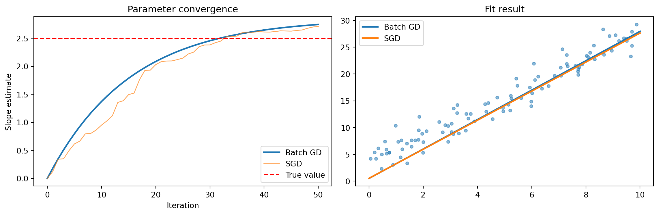
## Stochastic Gradient Descent (SGD)
SGD is the foundation of online learning. In classical gradient descent we compute the gradient on the **entire** dataset. In SGD — on a **single observation** (or small batch).
::: {.callout-tip collapse="true"}
## {{< fa mountain >}} Intuition: finding a path in the mountains
Imagine searching for the lowest point in the mountains in fog:
- **Gradient Descent** — you compute the terrain slope from a map of the entire mountains.
- **SGD** — you only look at your feet and take a step in the direction that looks steepest downhill.
Each SGD step is less precise, but you take **many more** of them and much faster.
:::
### Mathematically
**Gradient Descent (batch):**
$$\theta_{t+1} = \theta_t - \eta \cdot \frac{1}{N} \sum_{i=1}^{N} \nabla L_i(\theta_t)$$
**Stochastic Gradient Descent:**
$$\theta_{t+1} = \theta_t - \eta \cdot \nabla L_i(\theta_t)$$
where $\eta$ is the learning rate, and $i$ is a randomly selected observation.
**Mini-batch SGD** — a compromise: compute the gradient on a small sample (e.g., 32–256 observations):
$$\theta_{t+1} = \theta_t - \eta \cdot \frac{1}{|B|} \sum_{i \in B} \nabla L_i(\theta_t)$$
```{python}
#| label: fig-sgd-convergence
#| fig-cap: "SGD vs Batch GD — convergence and fit result"
import matplotlib.pyplot as plt

# Visualization: SGD vs Batch GD on a simple regression problem
np.random.seed(42)
X_reg = np.random.uniform(0, 10, 100)
y_reg = 2.5 * X_reg + 3 + np.random.normal(0, 2, 100)

# Batch GD
theta_batch = [0.0, 0.0]  # [slope, intercept]
lr = 0.001
batch_path = [tuple(theta_batch)]

for _ in range(50):
    pred = theta_batch[0] * X_reg + theta_batch[1]
    error = pred - y_reg
    theta_batch[0] -= lr * (2/len(X_reg)) * np.dot(error, X_reg)
    theta_batch[1] -= lr * (2/len(X_reg)) * np.sum(error)
    batch_path.append(tuple(theta_batch))

# SGD
theta_sgd = [0.0, 0.0]
sgd_path = [tuple(theta_sgd)]

for _ in range(50):
    i = np.random.randint(len(X_reg))
    pred_i = theta_sgd[0] * X_reg[i] + theta_sgd[1]
    error_i = pred_i - y_reg[i]
    theta_sgd[0] -= lr * 2 * error_i * X_reg[i]
    theta_sgd[1] -= lr * 2 * error_i
    sgd_path.append(tuple(theta_sgd))

fig, (ax1, ax2) = plt.subplots(1, 2, figsize=(12, 4))

batch_slopes = [p[0] for p in batch_path]
sgd_slopes = [p[0] for p in sgd_path]

ax1.plot(batch_slopes, label='Batch GD', linewidth=2)
ax1.plot(sgd_slopes, label='SGD', linewidth=1, alpha=0.7)
ax1.axhline(y=2.5, color='red', linestyle='--', label='True value')
ax1.set_xlabel('Iteration')
ax1.set_ylabel('Slope estimate')
ax1.set_title('Parameter convergence')
ax1.legend()

ax2.scatter(X_reg, y_reg, alpha=0.5, s=15)
ax2.plot([0, 10], [theta_batch[1], theta_batch[0]*10 + theta_batch[1]], label='Batch GD', linewidth=2)
ax2.plot([0, 10], [theta_sgd[1], theta_sgd[0]*10 + theta_sgd[1]], label='SGD', linewidth=2)
ax2.set_title('Fit result')
ax2.legend()

plt.tight_layout()
plt.show()
```
::: {.callout-note appearance="simple"}
SGD is "noisy" — but that's precisely its strength in online learning: each new observation immediately influences the model.
:::
---
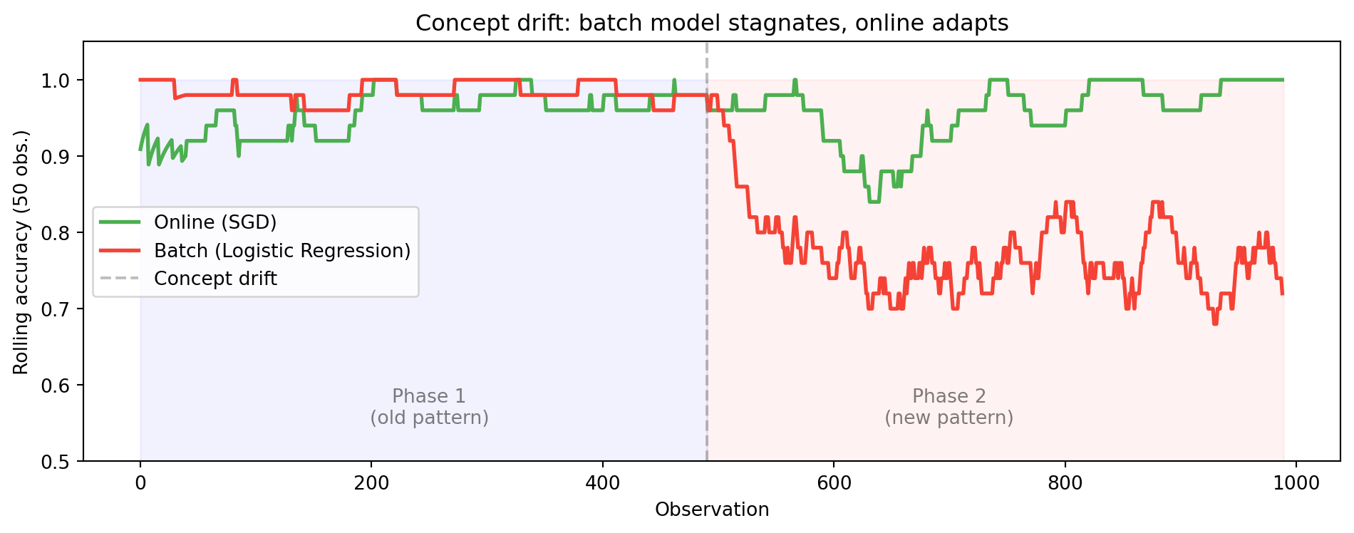
## Concept drift — when the world changes
::: {.callout-warning}
## Key challenge
**The data distribution changes over time** (concept drift). A model trained on last year's data may be useless today.
:::
### Types of drift
:::: {.columns}
::: {.column width="33%"}
::: {.callout-important appearance="simple"}
## {{< fa bolt >}} Sudden
E.g., a pandemic changes shopping patterns overnight.
:::
:::
::: {.column width="33%"}
::: {.callout-note appearance="simple"}
## {{< fa arrow-trend-up >}} Gradual
E.g., customer preferences change slowly over months.
:::
:::
::: {.column width="33%"}
::: {.callout-tip appearance="simple"}
## {{< fa rotate >}} Recurring
E.g., seasonal sales patterns.
:::
:::
::::
```{python}
# Simulation of concept drift: sudden change in pattern
np.random.seed(42)

# Phase 1: normal transactions (amount < 1000 = OK)
X_phase1 = np.random.uniform(10, 2000, 500).reshape(-1, 1)
y_phase1 = (X_phase1.ravel() > 1000).astype(int)

# Phase 2: after change — suspicion threshold drops to 500
X_phase2 = np.random.uniform(10, 2000, 500).reshape(-1, 1)
y_phase2 = (X_phase2.ravel() > 500).astype(int)

from sklearn.preprocessing import StandardScaler
scaler = StandardScaler()

# Batch model — trained on phase 1
model_batch = LogisticRegression()
model_batch.fit(scaler.fit_transform(X_phase1), y_phase1)
acc_batch_p2 = accuracy_score(y_phase2, model_batch.predict(scaler.transform(X_phase2)))

# Online model — adapts
model_sgd = SGDClassifier(loss='log_loss')
model_sgd.fit(scaler.transform(X_phase1), y_phase1)

# Online training on phase 2
for i in range(0, len(X_phase2), 10):
    X_b = scaler.transform(X_phase2[i:i+10])
    y_b = y_phase2[i:i+10]
    model_sgd.partial_fit(X_b, y_b)

acc_online_p2 = accuracy_score(y_phase2, model_sgd.predict(scaler.transform(X_phase2)))

print(f"After concept drift:")
print(f"  Batch model accuracy:  {acc_batch_p2:.3f}")
print(f"  Online model accuracy: {acc_online_p2:.3f}")
```
```{python}
#| label: fig-concept-drift
#| fig-cap: "Concept drift: batch vs online model — accuracy over time"
# Rolling accuracy simulation
from collections import deque

np.random.seed(42)
X_all = np.vstack([X_phase1, X_phase2])
y_all = np.concatenate([y_phase1, y_phase2])
X_all_s = scaler.fit_transform(X_all)

online = SGDClassifier(loss='log_loss')
batch = LogisticRegression()
batch.fit(X_all_s[:500], y_all[:500])

window = deque(maxlen=50)
online_acc, batch_acc = [], []

for i in range(len(X_all)):
    x_i = X_all_s[i:i+1]
    y_i = y_all[i:i+1]

    if i == 0:
        online.partial_fit(x_i, y_i, classes=[0, 1])
    else:
        pred_o = online.predict(x_i)[0]
        pred_b = batch.predict(x_i)[0]
        window.append((pred_o == y_i[0], pred_b == y_i[0]))
        online.partial_fit(x_i, y_i)

    if len(window) > 10:
        online_acc.append(np.mean([w[0] for w in window]))
        batch_acc.append(np.mean([w[1] for w in window]))

fig, ax = plt.subplots(figsize=(10, 4))
ax.plot(online_acc, label='Online (SGD)', color='#4CAF50', linewidth=2)
ax.plot(batch_acc, label='Batch (Logistic Regression)', color='#F44336', linewidth=2)
ax.axvline(x=490, color='gray', linestyle='--', alpha=0.5, label='Concept drift')
ax.fill_betweenx([0, 1], 0, 490, alpha=0.05, color='blue')
ax.fill_betweenx([0, 1], 490, len(online_acc), alpha=0.05, color='red')
ax.text(250, 0.55, 'Phase 1\n(old pattern)', ha='center', fontsize=10, alpha=0.5)
ax.text(700, 0.55, 'Phase 2\n(new pattern)', ha='center', fontsize=10, alpha=0.5)
ax.set_xlabel('Observation')
ax.set_ylabel('Rolling accuracy (50 obs.)')
ax.set_title('Concept drift: batch model stagnates, online adapts')
ax.set_ylim(0.5, 1.05)
ax.legend()
plt.tight_layout()
plt.show()
```
---
## Anomaly detection
::: {.callout-important appearance="simple"}
Anomaly detection is one of the **most important applications** of real-time data analytics. An anomaly (outlier) is an observation significantly distant from the rest of the data.
:::
::: {.panel-tabset}
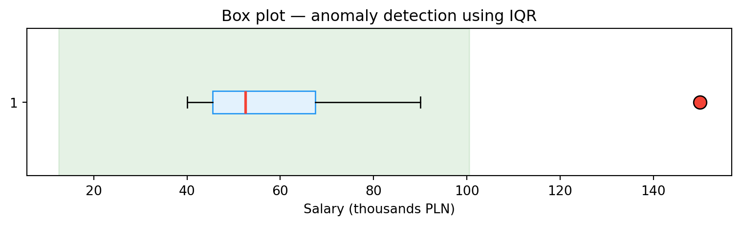
### IQR method
For a single variable we can use the interquartile range:
$$x_{\text{out}} < Q_1 - 1.5 \times IQR \quad \text{or} \quad x_{\text{out}} > Q_3 + 1.5 \times IQR$$
```{python}
salaries = [40, 42, 45, 47, 50, 55, 60, 70, 90, 150]

Q1 = np.percentile(salaries, 25)
Q3 = np.percentile(salaries, 75)
IQR = Q3 - Q1

lower_bound = Q1 - 1.5 * IQR
upper_bound = Q3 + 1.5 * IQR

outliers = [x for x in salaries if x < lower_bound or x > upper_bound]
print(f"Q1={Q1}, Q3={Q3}, IQR={IQR}")
print(f"Bounds: [{lower_bound:.1f}, {upper_bound:.1f}]")
print(f"Anomalies: {outliers}")

fig, ax = plt.subplots(figsize=(8, 2.5))
bp = ax.boxplot(salaries, vert=False, patch_artist=True,
                boxprops=dict(facecolor='#E3F2FD', edgecolor='#2196F3'),
                medianprops=dict(color='#F44336', linewidth=2),
                flierprops=dict(marker='o', markerfacecolor='#F44336', markersize=10))
ax.set_xlabel('Salary (thousands PLN)')
ax.set_title('Box plot — anomaly detection using IQR')
ax.axvspan(lower_bound, upper_bound, alpha=0.1, color='green', label='Normal range')
plt.tight_layout()
plt.show()
```
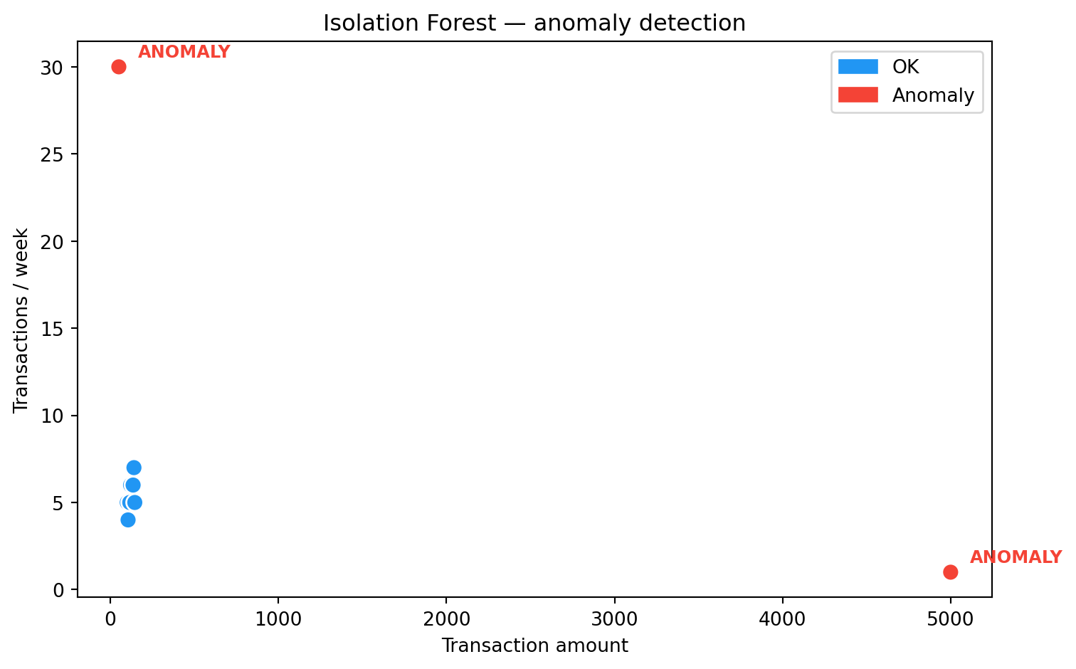
### Isolation Forest
A tree-based algorithm (Liu et al., 2008). Key intuition: **anomalies are easier to isolate** — random splits separate them from the rest of the data faster.
```{python}
from sklearn.ensemble import IsolationForest

# Simulation: banking transactions (amount, weekly frequency)
data = np.array([
    [100, 5], [120, 6], [130, 5], [110, 4], [125, 5],
    [115, 5], [140, 7], [135, 6], [145, 5], [105, 4],
    [5000, 1],  # anomaly: large amount, rare
    [50, 30],   # anomaly: small amount, very frequent
])

clf = IsolationForest(contamination=0.15, random_state=42)
predictions = clf.fit_predict(data)

df = pd.DataFrame(data, columns=["Amount", "Transactions/week"])
df["Status"] = ["Anomaly" if p == -1 else "OK" for p in predictions]
print(df.to_string(index=False))

colors = ['#F44336' if s == 'Anomaly' else '#2196F3' for s in df['Status']]
fig, ax = plt.subplots(figsize=(8, 5))
ax.scatter(df['Amount'], df['Transactions/week'], c=colors, s=80, edgecolors='white', zorder=5)
for _, row in df[df['Status'] == 'Anomaly'].iterrows():
    ax.annotate('ANOMALY', (row['Amount'], row['Transactions/week']),
                textcoords="offset points", xytext=(10, 5), fontsize=9, color='#F44336', fontweight='bold')
ax.set_xlabel('Transaction amount')
ax.set_ylabel('Transactions / week')
ax.set_title('Isolation Forest — anomaly detection')
import matplotlib.patches as mpatches
ax.legend(handles=[mpatches.Patch(color='#2196F3', label='OK'),
                    mpatches.Patch(color='#F44336', label='Anomaly')])
plt.tight_layout()
plt.show()
```
### In a stream
In a real-time context we can't analyze the entire dataset — we must detect anomalies **on the fly**, within a time window. In the labs we'll build such a system with Kafka and Spark.
:::
---
## Model explainability
::: {.callout-important}
## Regulations require transparency
In regulated industries (banking, insurance, medicine) it's not enough to say "the model rejected the loan application". You need to explain **why**. Regulations such as the **AI Act** and **GDPR** require transparency in algorithmic decisions.
:::
### LIME (Local Interpretable Model-Agnostic Explanations)
LIME explains individual predictions of any model. It works by introducing small changes to the input data and observing how the result changes. Based on this, it builds a simple, interpretable local model (e.g., linear regression) that approximates the behavior of the original model in the neighborhood of the given observation.
```{python}
from sklearn.ensemble import RandomForestClassifier
from sklearn.datasets import load_iris

iris = load_iris()
X_iris, y_iris = iris.data, iris.target
X_tr, X_te, y_tr, y_te = train_test_split(X_iris, y_iris, test_size=0.2, random_state=42)

rf = RandomForestClassifier(n_estimators=100, random_state=42)
rf.fit(X_tr, y_tr)

# Feature importance — simpler alternative to LIME
importances = pd.Series(rf.feature_importances_, index=iris.feature_names)
print("Feature importance (Random Forest):")
print(importances.sort_values(ascending=False).round(3))
print(f"\nIn the labs we'll install the LIME library and explore local explanations.")
```
---
## Summary
Batch and incremental learning are two complementary approaches. In practice they are often combined: a base model trained in batch mode is gradually updated in online mode. SGD enables learning on a data stream, but requires attention to concept drift and stability.
Anomaly detection and model explainability are key applications of ML in real-time analytics — in the labs we'll translate them into practical systems with Kafka and Spark.
::: {.callout-note appearance="simple"}
## {{< fa forward >}} Next lecture
Apache Kafka — architecture, producers, consumers, topics, partitions.
:::
::: {.callout-tip appearance="simple"}
## {{< fa brain >}} Food for thought
Your bank trains a fraud detection model once a month (batch). What business risk does this approach carry? What would change if the model learned online?
:::