przypomnienie - dane ustruktyryzowane

import numpy as np
import pandas as pd
from sklearn.model_selection import train_test_split

df = pd.read_csv("titanic.csv")

df.head()

	pclass	survived	name	sex	age	sibsp	parch	ticket	fare	cabin	embarked	boat	body	home.dest
0	1	1	Allen, Miss. Elisabeth Walton	female	29.0000	0	0	24160	211.3375	B5	S	2	NaN	St Louis, MO
1	1	1	Allison, Master. Hudson Trevor	male	0.9167	1	2	113781	151.5500	C22 C26	S	11	NaN	Montreal, PQ / Chesterville, ON
2	1	0	Allison, Miss. Helen Loraine	female	2.0000	1	2	113781	151.5500	C22 C26	S	NaN	NaN	Montreal, PQ / Chesterville, ON
3	1	0	Allison, Mr. Hudson Joshua Creighton	male	30.0000	1	2	113781	151.5500	C22 C26	S	NaN	135.0	Montreal, PQ / Chesterville, ON
4	1	0	Allison, Mrs. Hudson J C (Bessie Waldo Daniels)	female	25.0000	1	2	113781	151.5500	C22 C26	S	NaN	NaN	Montreal, PQ / Chesterville, ON

numeric_features = ['age', 'fare']
categorical_features = ['pclass', 'sex', 'embarked']

X = df[numeric_features + categorical_features].copy()
y = df['survived'].astype(int) # Cel: czy przeżył (0 lub 1)

X['useless_column'] = 'Taka Sama Wartosc'
categorical_features.append('useless_column')

X.head()

	age	fare	pclass	sex	embarked	useless_column
0	29.0000	211.3375	1	female	S	Taka Sama Wartosc
1	0.9167	151.5500	1	male	S	Taka Sama Wartosc
2	2.0000	151.5500	1	female	S	Taka Sama Wartosc
3	30.0000	151.5500	1	male	S	Taka Sama Wartosc
4	25.0000	151.5500	1	female	S	Taka Sama Wartosc

X_tr, X_test, y_tr, y_test = train_test_split(X, y, test_size=0.2, random_state=42)

X_tr.info()

<class 'pandas.core.frame.DataFrame'>
Index: 1047 entries, 772 to 1126
Data columns (total 6 columns):
 #   Column          Non-Null Count  Dtype  
---  ------          --------------  -----  
 0   age             840 non-null    float64
 1   fare            1046 non-null   float64
 2   pclass          1047 non-null   int64  
 3   sex             1047 non-null   object 
 4   embarked        1046 non-null   object 
 5   useless_column  1047 non-null   object 
dtypes: float64(2), int64(1), object(3)
memory usage: 57.3+ KB

from sklearn.pipeline import Pipeline
from sklearn.compose import ColumnTransformer
from sklearn.preprocessing import StandardScaler, OneHotEncoder
from sklearn.impute import SimpleImputer
from sklearn.linear_model import LogisticRegression
from sklearn.ensemble import RandomForestClassifier
from sklearn.base import BaseEstimator, TransformerMixin, ClassifierMixin

class DelOneValueFeature(BaseEstimator, TransformerMixin):
    def __init__(self):
        self.one_value_features = []

    def fit(self, X, y=None):
        if not isinstance(X, pd.DataFrame):
            X = pd.DataFrame(X)
        
        self.one_value_features = [col for col in X.columns if X[col].nunique() == 1]
        return self

    def transform(self, X, y=None):
        if not isinstance(X, pd.DataFrame):
            X = pd.DataFrame(X)
        if not self.one_value_features:
            return X
        return X.drop(columns=self.one_value_features)

class RandomClassifier(BaseEstimator, ClassifierMixin):
    def __init__(self, random_state=None):
        self.random_state = random_state
        self.classes_ = None

    def fit(self, X, y):
        # Zapamiętujemy unikalne klasy z wektora docelowego
        self.classes_ = np.unique(y)
        return self

    def predict(self, X):
        np.random.seed(self.random_state)
        # Losujemy klasy dla każdego wiersza w X
        return np.random.choice(self.classes_, size=len(X))

    def predict_proba(self, X):
        np.random.seed(self.random_state)
        # Losujemy prawdopodobieństwa, które sumują się do 1
        raw_probs = np.random.rand(len(X), len(self.classes_))
        return raw_probs / raw_probs.sum(axis=1, keepdims=True)

numeric_transformer = Pipeline(steps=[
    ("imputer", SimpleImputer(strategy="mean")),
    ("scaler", StandardScaler())
])

categorical_transformer = Pipeline(steps=[
    ("remover", DelOneValueFeature()),  # Usunie 'useless_column' przed OneHotEncoderem!
    ("imputer", SimpleImputer(strategy="most_frequent")),
    ("encoder", OneHotEncoder(handle_unknown="ignore", sparse_output=False))
])

preprocessor = ColumnTransformer(transformers=[
    ("num_trans", numeric_transformer, numeric_features),
    ("cat_trans", categorical_transformer, categorical_features)
])

full_pipeline = Pipeline(steps=[
    ("preproc", preprocessor),
    ("model", LogisticRegression())
])

param_grid = [
    # Siatka 1: Random Forest
    {
        "preproc__num_trans__imputer__strategy": ["mean", "median"],
        "model": [RandomForestClassifier(random_state=42)],
        "model__n_estimators": [10, 50, 100],
        "model__max_depth": [None, 5, 10]
    },
    # Siatka 2: Logistic Regression
    {
        "preproc__num_trans__imputer__strategy": ["mean", "median"],
        "model": [LogisticRegression(max_iter=1000)],
        "model__C": [0.1, 1.0, 10.0]
    },
    {
        "model": [RandomClassifier(random_state=42)]
    }
]

from sklearn.model_selection import GridSearchCV

grid_search = GridSearchCV(full_pipeline, param_grid, cv=3, verbose=1, n_jobs=-1)

grid_search.fit(X_tr, y_tr)

Fitting 3 folds for each of 25 candidates, totalling 75 fits

print("\n" + "="*40)
print("NAJLEPSZE PARAMETRY:")
print("="*40)
for param, val in grid_search.best_params_.items():
    print(f"{param}: {val}")

# Wynik na zbiorze testowym dla najlepszego modelu
best_model_score = grid_search.score(X_test, y_test)


========================================
NAJLEPSZE PARAMETRY:
========================================
model: RandomForestClassifier(random_state=42)
model__max_depth: 5
model__n_estimators: 100
preproc__num_trans__imputer__strategy: mean

best_model_score

0.7633587786259542

print("\n" + "="*40)
print("NAJLEPSZE PARAMETRY:")
print("="*40)
for param, val in grid_search.best_params_.items():
    print(f"{param}: {val}")

# Wynik na zbiorze testowym dla najlepszego modelu
best_model_score = grid_search.score(X_test, y_test)

# Sprawdźmy jak poradziłby sobie sam model losowy dla porównania
random_baseline = RandomClassifier(random_state=42)
random_baseline.fit(X_tr, y_tr)
random_score = random_baseline.score(X_test, y_test)

print("\n" + "="*40)
print("PORÓWNANIE DOKŁADNOŚCI (ACCURACY):")
print("="*40)
print(f"Nasz najlepszy model z GridSearch: {best_model_score:.4f}")
print(f"Model stricte losowy (Baseline):  {random_score:.4f}")


========================================
NAJLEPSZE PARAMETRY:
========================================
model: RandomForestClassifier(random_state=42)
model__max_depth: 5
model__n_estimators: 100
preproc__num_trans__imputer__strategy: mean

========================================
PORÓWNANIE DOKŁADNOŚCI (ACCURACY):
========================================
Nasz najlepszy model z GridSearch: 0.7634
Model stricte losowy (Baseline):  0.4847

Na poprzednich zajęciach omawialiśmy wykorzystanie modelu regresji liniowej dla danych ustrukturyzowanych. W najprostszym przypadku dla jednej zmiennej X i jednej zmiennej celu moglibyśmy np. przypisać model w postaci:

satysfakcja_z_zycia = $\alpha_0$ + $\alpha_1$ PKB_per_capita

$\alpha_0$ nazywamy punktem odcięcia (intercept) albo punktem obciążenia (bias)

import numpy as np

np.random.seed(42) 
m = 100
X = 2*np.random.rand(m,1) 
a_0, a_1 = 4, 3
y = a_0 + a_1 * X + np.random.randn(m,1)

import matplotlib.pyplot as plt

plt.scatter(X, y)
plt.show()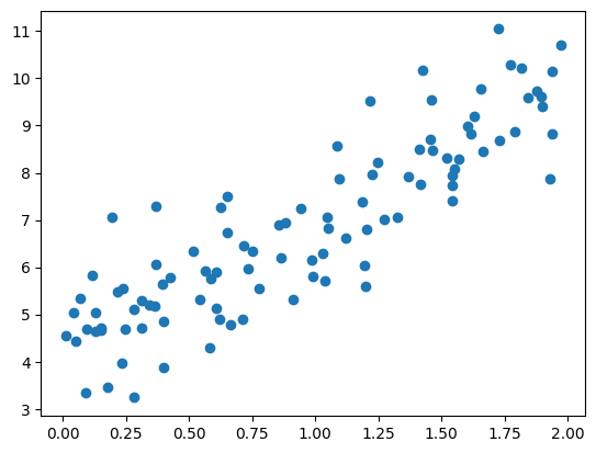

W ogólności model liniowy: $\hat{y} = \alpha_0 + \alpha_1 x_1 + \alpha_2 x_2 + \dots + \alpha_n x_n$ gdzie $\hat{y}$ to predykcja naszego modelu (wartość prognozowana), dla $n$ cech przy wartościach cechy $x_i$.

W postaci zwektoryzowanej możemy napisać: $\hat{y} = \vec{\alpha}^{T} \vec{x}$

W tej postaci widać dlaczego w tym modelu dokłada się kolumnę jedynek - wynikają one z wartości $x_0$ dla $\alpha_0$.

# dodajmy jedynkę do naszej tabeli 
from sklearn.preprocessing import add_dummy_feature

X_b = add_dummy_feature(X)

Powiedzieliśmy, że możemy w tym modelu znaleźć funkcję kosztu

$MSE(\vec{x}, \hat{y}) = \sum_{i=1}^{m} \left( \vec{\alpha}^{T} \vec{x}^{(i)} - y^{(i)} \right)^{2}$

Tak naprawdę możemy $MSE(\vec{x}, \hat{y}) = MSE(\vec{\alpha})$

Rozwiązanie analityczne: $\vec{\alpha} = (X^{T}X)^{-1} X^T y$

alpha_best = np.linalg.inv(X_b.T @ X_b) @ X_b.T @ y

alpha_best, np.array([4,3])

(array([[4.21509616],
        [2.77011339]]),
 array([4, 3]))

X_new = np.array([[0],[2]])

X_new_b = add_dummy_feature(X_new)

y_predict = X_new_b @ alpha_best

import matplotlib.pyplot as plt

plt.plot(X_new, y_predict, "r-", label="prediction")
plt.plot(X,y, "b.")
plt.show()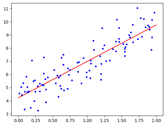

from sklearn.linear_model import LinearRegression
lin_reg = LinearRegression()
lin_reg.fit(X,y) 

print(f"a_0={lin_reg.intercept_[0]}, a_1 = {lin_reg.coef_[0][0]}")

print("predykcja", lin_reg.predict(X_new))

a_0=4.215096157546747, a_1 = 2.7701133864384837
predykcja [[4.21509616]
 [9.75532293]]

# Logistic Regression w scikit learn oparta jest o metodę lstsq 
alpha_best_svd, _, _, _ = np.linalg.lstsq(X_b, y, rcond=1e-6)
alpha_best_svd

array([[4.21509616],
       [2.77011339]])

Gradient prosty

Pamiętaj o standaryzacji zmiennych (aby były one reprezentowane w tej samej skali).

Wsadowy gradient prosty

W celu implementacji musimy policzyć pochodne cząstkowe dla funkcji kosztu wobec każdego parametru $\alpha_i$.

$\frac{\partial}{\partial \alpha_j}MSE(\vec{x}, \hat{y}) = 2 \sum_{i=1}^{m} \left( \vec{\alpha}^{T} \vec{x}^{(i)} - y^{(i)} \right) x_j^{(i)}$

Komputery posiadają własność mnożenia macierzy co pozwala obliczyć nam wszystkie pochodne w jednym obliczeniu. Wzór i algorytm liczący wszystkie pochodne “na raz” wykorzystuje cały zbiór X dlatego też nazywamy go wsadowym.

Po obliczeniu gradientu po prostu idziemy “w przeciwną stronę”

$ {next} = - {} MSE()$

from IPython.display import Image

Image(filename='02_10.png', width=500)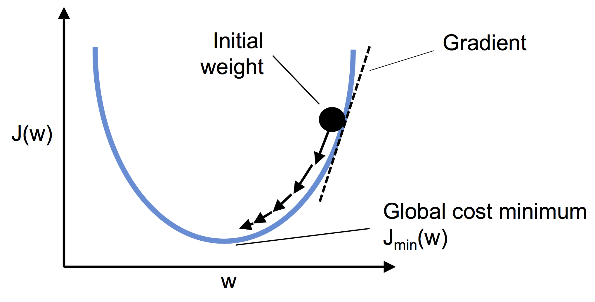

eta = 0.1
n_epochs = 1000
m = len(X_b)
np.random.seed(42) 
alpha = np.random.randn(2,1) # losowo wybieramy rozwiązanie
print(f"alpha init {alpha}")
for epoch in range(n_epochs):
    gradients = 2/m* X_b.T @ (X_b @ alpha - y)
    #print(alpha)
    alpha = alpha - eta*gradients

alpha init [[ 0.49671415]
 [-0.1382643 ]]

alpha

array([[4.21509616],
       [2.77011339]])

Stochastic gradient descent

Jednym z poważniejszych problemów wsadowego gradientu jest jego zależność od wykorzystania (w każdym kroku) całej macierzy danych. Korzystając z własności statystycznych możemy zobaczyć jak będzie realizowała się zbieżność rozwiązania jeśli za każdym razem wylosujemy próbkę danych i na niej określimy gradient. Ze względu, iż w pamięci przechowujemy tylko pewną porcję danych algorytm ten może być używany dla bardzo dużych zbiorów danych. Warto jednak mieć świadomość, że tak otrzymane wyniki mają charakter chaotyczny, co oznacza, że funkcja kosztu nie zbiega się w kierunku minimum lecz przeskakuje dążąc do minimun w sensie średniej.

n_epochs = 50
m = len(X_b)


def learning_schedule(t, t0=5, t1=50):
    return t0/(t+t1)

np.random.seed(42)
alpha = np.random.randn(2,1)

for epoch in range(n_epochs):
    for iteration in range(m):
        random_index = np.random.randint(m)
        xi = X_b[random_index : random_index + 1]
        yi = y[random_index : random_index + 1] 
        gradients = 2 * xi.T @ (xi @ alpha - yi)
        eta = learning_schedule(epoch * m + iteration) 
        alpha = alpha - eta * gradients

alpha

array([[4.21076011],
       [2.74856079]])

from sklearn.linear_model import SGDRegressor

sgd_reg = SGDRegressor(max_iter=1000, tol=1e-5, 
                       penalty=None, eta0=0.01, 
                       n_iter_no_change=100, random_state=42)

sgd_reg.fit(X, y.ravel())

SGDRegressor(n_iter_no_change=100, penalty=None, random_state=42, tol=1e-05)

In a Jupyter environment, please rerun this cell to show the HTML representation or trust the notebook.
On GitHub, the HTML representation is unable to render, please try loading this page with nbviewer.org.

sgd_reg.intercept_, sgd_reg.coef_

(array([4.21278812]), array([2.77270267]))

from random import randint
randint(1,6)

from random import randint

class Kosc():
    """ opis """
    def __init__(self, sciany=6):
        """
        to jest metoda do uruchamiania podczas inicjalizacji obiektu
        params: 
        sciany (int)

        """
        self.sciany = sciany

    def roll(self):
        """ opis"""
        return randint(1, self.sciany)

a = Kosc(sciany=12)
[a.roll() for _ in range(10)]

[6, 12, 7, 1, 3, 1, 1, 2, 3, 5]

from random import choice
choice([0,1,2,3,4])

from random import choice

class RandomWalk():
    def __init__(self, num_points=5000):
        self.num_points = num_points
        self.x_values = [0]
        self.y_values = [0]

    def fill_walk(self):
        while len(self.x_values) < self.num_points:
            # ruch prawo-lewo 
            # wylosuj kierunek dodatni lub ujemy oraz odległość 0-5 i przypisz do zmiennych
            
            x_direction = choice([-1,1])
            x_distance = choice([0,1,2,3,4])
            x_step = x_direction*x_distance
            
            y_direction = choice([-1,1])
            y_distance = choice([0,1,2,3,4])
            y_step = y_direction*y_distance
            
            # napisz warunek pomijający krok gdy x i y step = 0 (użyj continue)
            if x_step == 0 and y_step == 0:
                continue
            
            next_x = self.x_values[-1] + x_step
            next_y = self.y_values[-1] + y_step
            
            self.x_values.append(next_x)
            self.y_values.append(next_y)

rw = RandomWalk(10000)
rw.fill_walk()

rw.x_values[:5]

[0, 4, 4, 8, 10]

import matplotlib.pyplot as  plt
point_number = list(range(rw.num_points))
plt.scatter(rw.x_values, rw.y_values, c=point_number, cmap=plt.cm.Blues,
           edgecolor='none', s=15)
plt.scatter(0,0,c='green', edgecolor='none', s=100)
plt.scatter(rw.x_values[-1], rw.y_values[-1],c='red', edgecolor='none', s=100)

plt.show()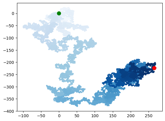

import numpy as np
import pandas as pd
from sklearn.datasets import load_iris

iris = load_iris()
df = pd.DataFrame(data= np.c_[iris['data'], iris['target']],
                  columns= iris['feature_names'] + ['target'])

X = df.iloc[:100,[0,2]].values
y = df.iloc[0:100,4].values
y = np.where(y == 0, -1, 1)

import matplotlib.pyplot as plt

plt.scatter(X[:50,0],X[:50,1],color='red', marker='o',label='setosa')
plt.scatter(X[50:100,0],X[50:100,1],color='blue', marker='x',label='versicolor')
plt.xlabel('sepal length (cm)')
plt.ylabel('petal length (cm)')
plt.legend(loc='upper left')
plt.show()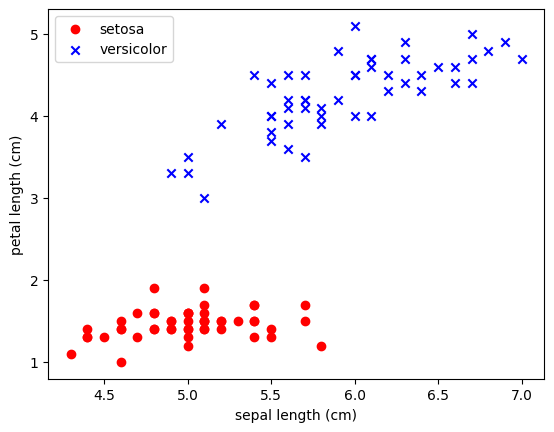

dziecko = Perceptron() dziecko.fit()

dziecko musi mieć parametr uczenia

dziecko.eta

możemy sprawdzić jak szybko się uczy == ile błędów robi

dziecko.errors_

rozwiązania znajdą się w wagach

dziecko.w_ # w naszym przypadku dziecko uczy się dwóch wag !

Image(filename='02_01.png', width=800)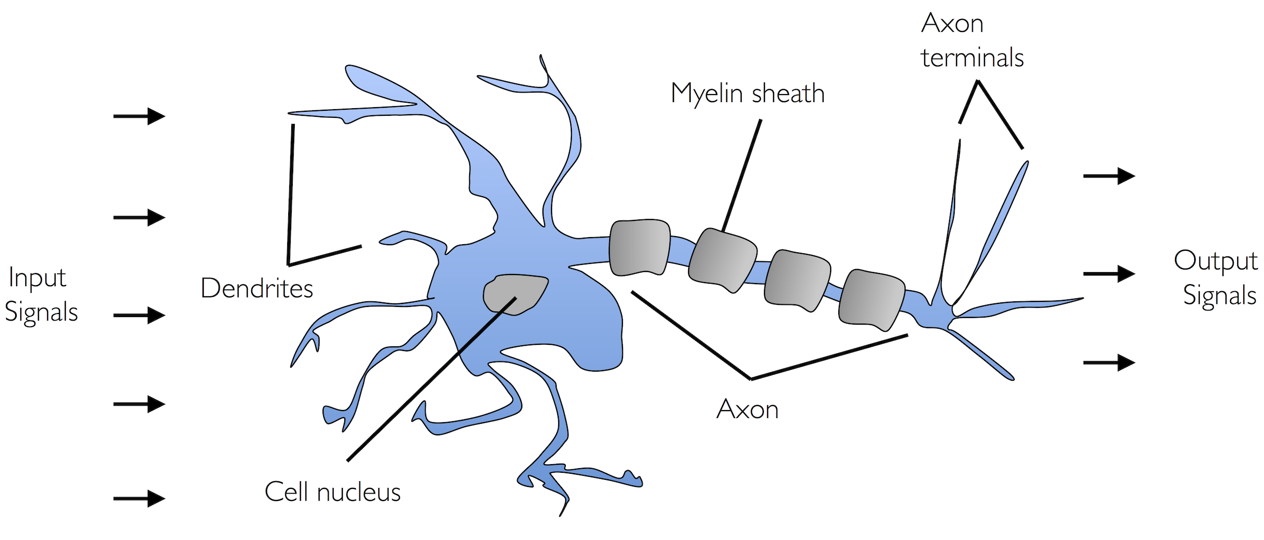

Image(filename='02_04.png', width=800)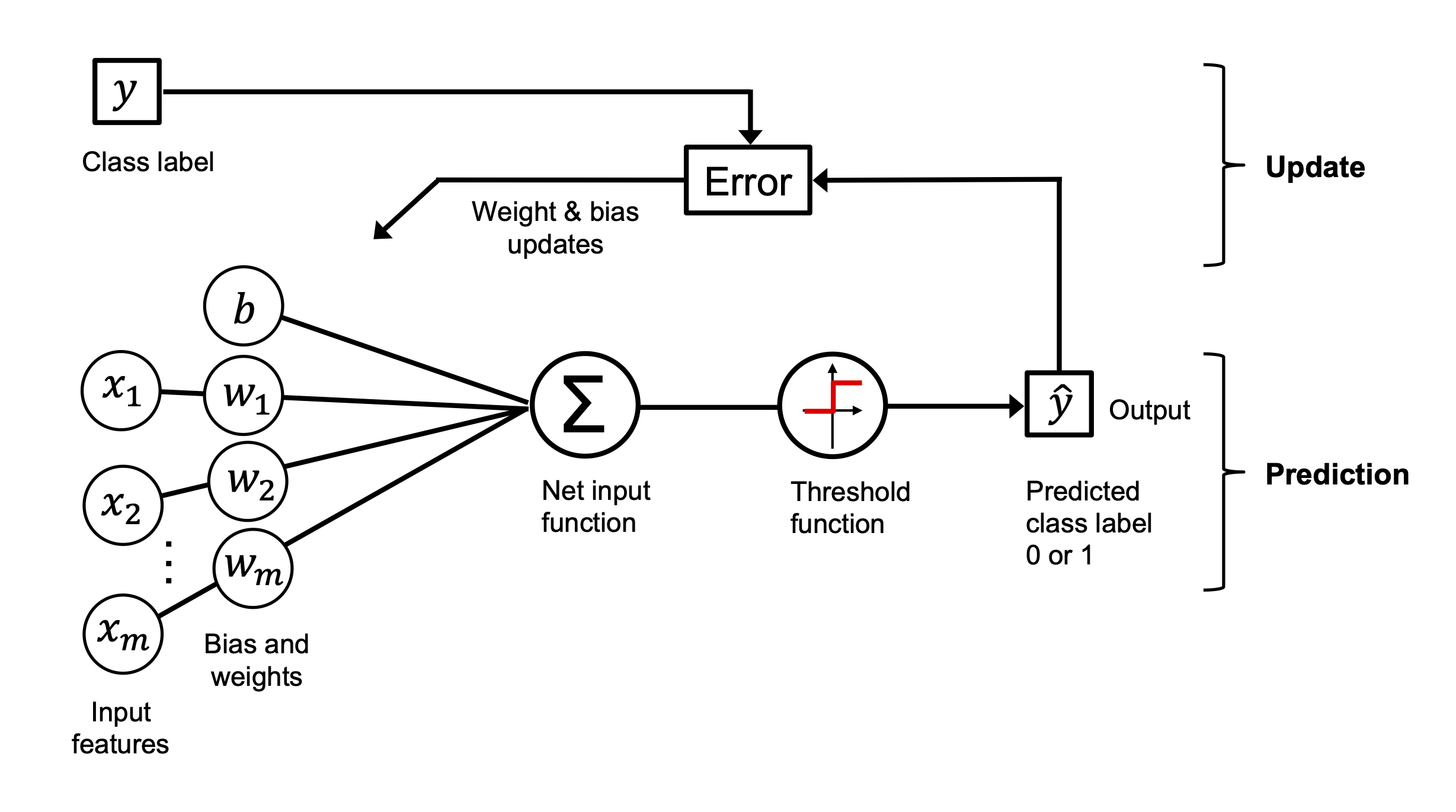

Image(filename='02_02.png', width=800)

class Perceptron():
    def __init__(self, n_iter=10, eta=0.01):
        self.n_iter = n_iter
        self.eta = eta
        
    def fit(self, X, y):
        self.w_ = np.zeros(1+X.shape[1])
        self.errors_ = []
        for _ in range(self.n_iter):
            pass
        return self

import random

class Perceptron():
    
    def __init__(self, eta=0.01, n_iter=10):
        self.eta = eta
        self.n_iter = n_iter
    
    def fit(self, X, y):
        
        #self.w_ = np.zeros(1+X.shape[1])
        self.w_ = [random.uniform(-1.0, 1.0) for _ in range(1+X.shape[1])] 
        self.errors_ = []
        
        for _ in range(self.n_iter):
            errors = 0
            for xi, target in zip(X,y):
                #print(xi, target)
                update = self.eta*(target-self.predict(xi))
                #print(update)
                self.w_[1:] += update*xi
                self.w_[0] += update
                #print(self.w_)
                errors += int(update != 0.0)
            self.errors_.append(errors)
        return self
    
    def net_input(self, X):
        return np.dot(X, self.w_[1:])+self.w_[0]
    
    def predict(self, X):
        return np.where(self.net_input(X)>=0.0, 1, -1)

ppn = Perceptron()
ppn.fit(X,y)

<__main__.Perceptron at 0xffff501b1990>

print(ppn.errors_)
print(ppn.w_)

[2, 3, 2, 3, 1, 0, 0, 0, 0, 0]
[np.float64(0.8281724951930811), np.float64(-0.3278624665243334), np.float64(0.3708385651137017)]

ppn.predict(np.array([-3, 5]))

array(1)

from matplotlib.colors import ListedColormap

def plot_decision_regions(X,y,classifier, resolution=0.02):
    markers = ('s','x','o','^','v')
    colors = ('red','blue','lightgreen','gray','cyan')
    cmap = ListedColormap(colors[:len(np.unique(y))])

    x1_min, x1_max = X[:,0].min() - 1, X[:,0].max()+1
    x2_min, x2_max = X[:,1].min() -1, X[:,1].max()+1
    xx1, xx2 = np.meshgrid(np.arange(x1_min, x1_max, resolution),
                           np.arange(x2_min, x2_max, resolution))
    Z = classifier.predict(np.array([xx1.ravel(), xx2.ravel()]).T)
    Z = Z.reshape(xx1.shape)
    plt.contourf(xx1, xx2, Z, alpha=0.4, cmap=cmap)
    plt.xlim(xx1.min(), xx1.max())
    plt.ylim(xx2.min(),xx2.max())

    for idx, cl in enumerate(np.unique(y)):
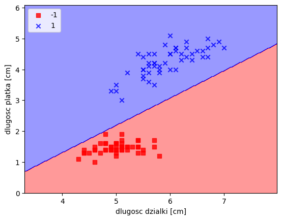
        plt.scatter(x=X[y == cl,0], y=X[y==cl,1], alpha=0.8, color=cmap(idx), marker=markers[idx], label=cl)

plot_decision_regions(X,y,classifier=ppn)
plt.xlabel("dlugosc dzialki [cm]")
plt.ylabel("dlugosc platka [cm]")
plt.legend(loc='upper left')
plt.show()