Python OOP - Percepron Class

from IPython.display import Image

Structured data

During the previous classes, we discussed the use of linear regression model for structured data. In the simplest case, for one variable X and one target variable, we could, for example, assign the model in the form:

life_satisfaction = \(\alpha_0\) + \(\alpha_1\) GDP_per_capita

We call \(\alpha_0\) the intercept or bias term.

import numpy as np

np.random.seed(42) 
m = 100
X = 2*np.random.rand(m,1) 
a_0, a_1 = 4, 3 
y = a_0 + a_1 * X + np.random.randn(m,1) 

import matplotlib.pyplot as plt

plt.scatter(X, y)
plt.show()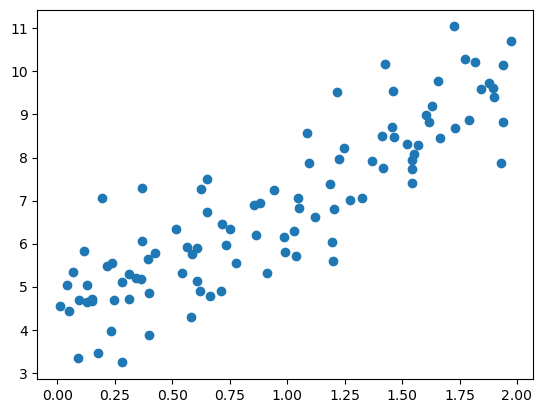

In general, the linear model is represented as:

\(\hat{y} = \alpha_0 + \alpha_1 x_1 + \alpha_2 x_2 + \dots + \alpha_n x_n\)

where \(\hat{y}\) is the prediction of our model (predicted value) for \(n\) features with values \(x_i\).

In vectorized form, we can write:

\(\hat{y} = \vec{\alpha}^{T} \vec{x}\)

In this form, it is evident why a column of ones is added to this model - they correspond to the values \(x_0\) for \(\alpha_0\).

# add ones 
from sklearn.preprocessing import add_dummy_feature

X_b = add_dummy_feature(X)

We said that in this model, we can find a cost function.

\(MSE(\vec{x}, \hat{y}) = \sum_{i=1}^{m} \left( \vec{\alpha}^{T} \vec{x}^{(i)} - y^{(i)} \right)^{2}\)

Actually, we can have \(MSE(\vec{x}, \hat{y}) = MSE(\vec{\alpha})\).

Analytical solution \(\vec{\alpha} = (X^{T}X)^{-1} X^T y\)

# solution
alpha_best = np.linalg.inv(X_b.T @ X_b) @ X_b.T @ y

alpha_best, np.array([4,3])

(array([[4.21509616],
        [2.77011339]]),
 array([4, 3]))

X_new = np.array([[0],[2]])
X_new_b = add_dummy_feature(X_new)
y_predict = X_new_b @ alpha_best

import matplotlib.pyplot as plt

plt.plot(X_new, y_predict, "r-", label="prediction")
plt.plot(X,y, "b.")
plt.show()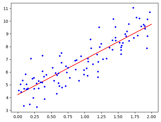

from sklearn.linear_model import LinearRegression
lin_reg = LinearRegression()
lin_reg.fit(X,y) 

print(f"a_0={lin_reg.intercept_[0]}, a_1 = {lin_reg.coef_[0][0]}")

print("prediction", lin_reg.predict(X_new))

a_0=4.215096157546746, a_1 = 2.770113386438484
prediction [[4.21509616]
 [9.75532293]]

# Logistic Regression w scikit learn oparta jest o metodę lstsq 
alpha_best_svd, _, _, _ = np.linalg.lstsq(X_b, y, rcond=1e-6)
alpha_best_svd

array([[4.21509616],
       [2.77011339]])

Remember about variable standardization (to represent them on the same scale).

Batch Gradient Descent

For implementation, we need to calculate partial derivatives for the cost function with respect to each parameter \(\alpha_i\).

\(\frac{\partial}{\partial \alpha_j}MSE(\vec{x}, \hat{y}) = 2 \sum_{i=1}^{m} \left( \vec{\alpha}^{T} \vec{x}^{(i)} - y^{(i)} \right) x_j^{(i)}\)

Computers have the property of matrix multiplication, which allows us to calculate all derivatives in one computation. The formula and algorithm calculating all derivatives “at once” use the entire set X, hence we call it batch.

After calculating the gradient, we simply go “in the opposite direction”.

$ {next} = - {} MSE()$

Image(filename='./img/02_10.png', width=500)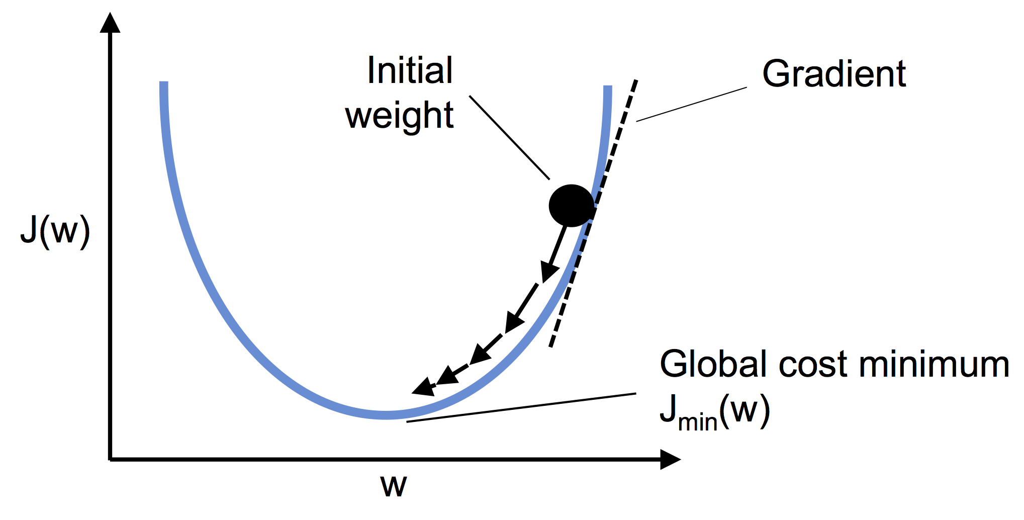

eta = 0.1
n_epochs = 1000
m = len(X_b)
np.random.seed(42) 
alpha = np.random.randn(2,1) # losowo wybieramy rozwiązanie

for epoch in range(n_epochs):
    gradients = 2/m* X_b.T @ (X_b @ alpha - y)
    #print(alpha)
    alpha = alpha - eta*gradients

alpha

array([[4.21509616],
       [2.77011339]])

verify for eta 0.02, 0.1, 0.5

Now a minor modification - we know that we don’t want such a variable in the model - it has only one value. But how to verify which variables are these if you have 3 million columns?

Stochastic gradient descent

One of the more serious problems with batch gradient is its dependence on using the entire data matrix (at each step). By utilizing statistical properties, we can observe how the convergence of the solution will proceed if we randomly draw a data sample each time and determine the gradient on it. Due to the fact that we store only a certain portion of the data in memory, this algorithm can be used for very large datasets. However, it is worth noting that the results obtained in this way are chaotic, which means that the cost function does not converge towards the minimum but rather jumps around, aiming towards the minimum in the sense of average.

n_epochs = 50
m = len(X_b)


def learning_schedule(t, t0=5, t1=50):
    return t0/(t+t1)

np.random.seed(42)
alpha = np.random.randn(2,1)

for epoch in range(n_epochs):
    for iteration in range(m):
        random_index = np.random.randint(m)
        xi = X_b[random_index : random_index + 1]
        yi = y[random_index : random_index + 1] 
        gradients = 2 * xi.T @ (xi @ alpha - yi)
        eta = learning_schedule(epoch * m + iteration) 
        alpha = alpha - eta * gradients
        

alpha

array([[4.21076011],
       [2.74856079]])

from sklearn.linear_model import SGDRegressor

sgd_reg = SGDRegressor(max_iter=1000, tol=1e-5, 
                       penalty=None, eta0=0.01, 
                       n_iter_no_change=100, random_state=42)

sgd_reg.fit(X, y.ravel())

SGDRegressor(n_iter_no_change=100, penalty=None, random_state=42, tol=1e-05)

In a Jupyter environment, please rerun this cell to show the HTML representation or trust the notebook.
On GitHub, the HTML representation is unable to render, please try loading this page with nbviewer.org.

sgd_reg.intercept_, sgd_reg.coef_

(array([4.21278812]), array([2.77270267]))

Perceptron and Python OOP

from random import randint

class Dice():
    """class descr"""
    def __init__(self, sciany=6):
        """ init descr """
        self.sciany = sciany
        
    def roll(self):
        """roll descr """
        return randint(1,self.sciany)

a = Dice()
[a.roll() for _ in range(10)]

[2, 6, 6, 3, 1, 6, 4, 2, 6, 5]

from random import choice

class RandomWalk():
    def __init__(self, num_points=5000):
        self.num_points = num_points
        self.x_values = [0]
        self.y_values = [0]
    
    def fill_walk(self):
        while len(self.x_values) < self.num_points:
            x_direction = choice([-1,1])
            x_distance = choice([0,1,2,3,4])
            x_step = x_direction*x_distance
            
            y_direction = choice([-1,1])
            y_distance = choice([0,1,2,3,4])
            y_step = y_direction*y_distance
            
            if x_step == 0 and y_step == 0:
                continue
            
            next_x = self.x_values[-1] + x_step
            next_y = self.y_values[-1] + y_step
            
            self.x_values.append(next_x)
            self.y_values.append(next_y)

rw = RandomWalk()
rw.x_values
rw2 = RandomWalk(num_points=10000)
rw2.num_points

rw.fill_walk()

import matplotlib.pyplot as  plt
point_number = list(range(rw.num_points))
plt.scatter(rw.x_values, rw.y_values, c=point_number, cmap=plt.cm.Blues,
           edgecolor='none', s=15)
plt.scatter(0,0,c='green', edgecolor='none', s=100)
plt.scatter(rw.x_values[-1], rw.y_values[-1],c='red', edgecolor='none', s=100)

plt.show()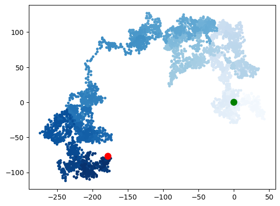

Sztuczne neurony - rys historyczny

In 1943, W. McCulloch and W. Pitts presented the first concept of a simplified model of a nerve cell called the McCulloch-Pitts Neuron (MCP). W.S. McCulloch, W. Pitts, A logical Calculus of the Ideas Immanent in Nervous Activity. “The Bulletin of Mathematical Biophysics” 1943 nr 5(4)

Neurons are mutually connected nerve cells in the brain responsible for processing and transmitting chemical and electrical signals. Such a cell is described as a logical gate containing binary outputs. A large number of signals reach the dendrites, which are integrated in the cell body and (if the energy exceeds a certain threshold value) generate an output signal transmitted through the axon.

Image(filename='./img/02_01.png', width=800)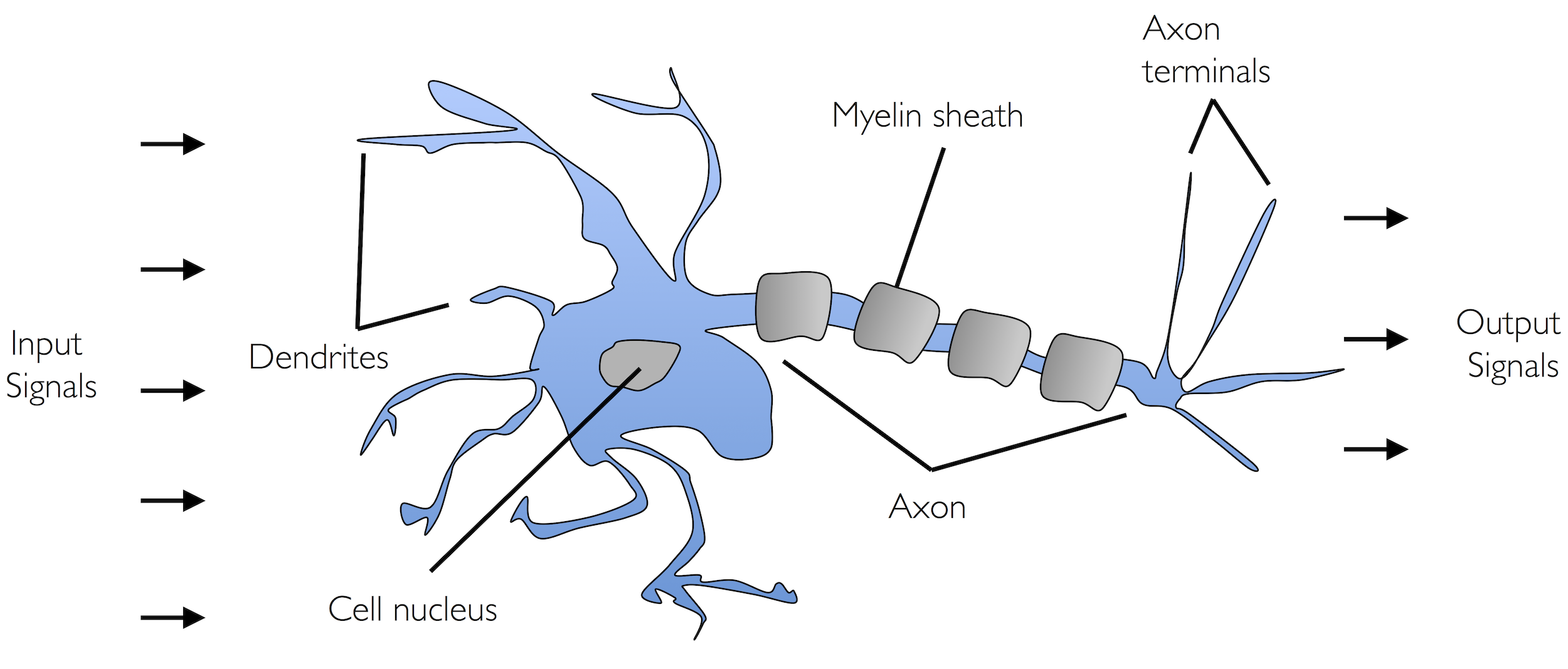 

After several years, Frank Rosenblatt (based on the MCP) proposed the first concept of the perceptron learning rule. F. Rosenblatt, The Perceptron, a Perceiving and Recognizing Automaton, Cornell Aeronautical Laboratory, 1957

 Image(filename='./img/02_04.png', width=800)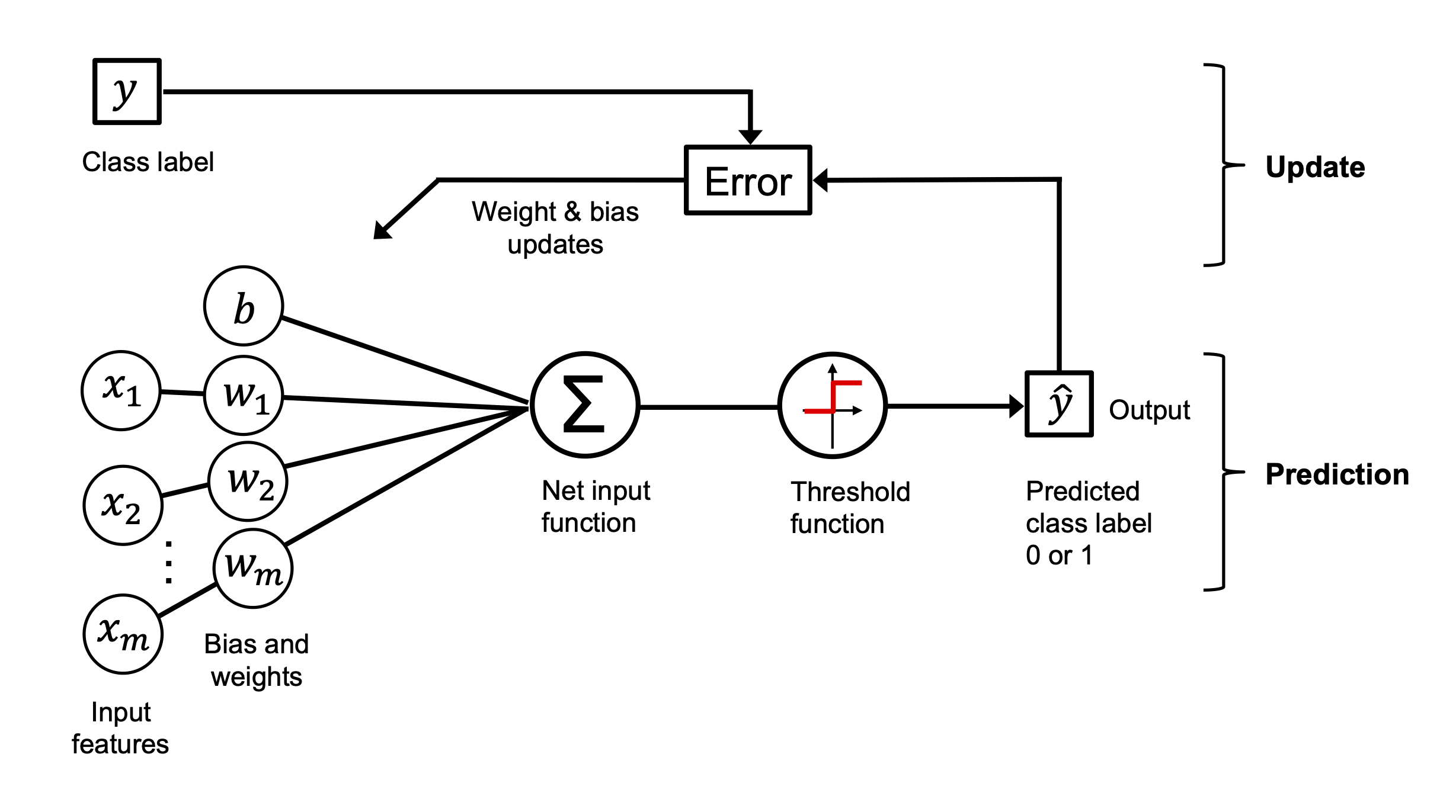 

Image(filename='./img/02_02.png', width=800)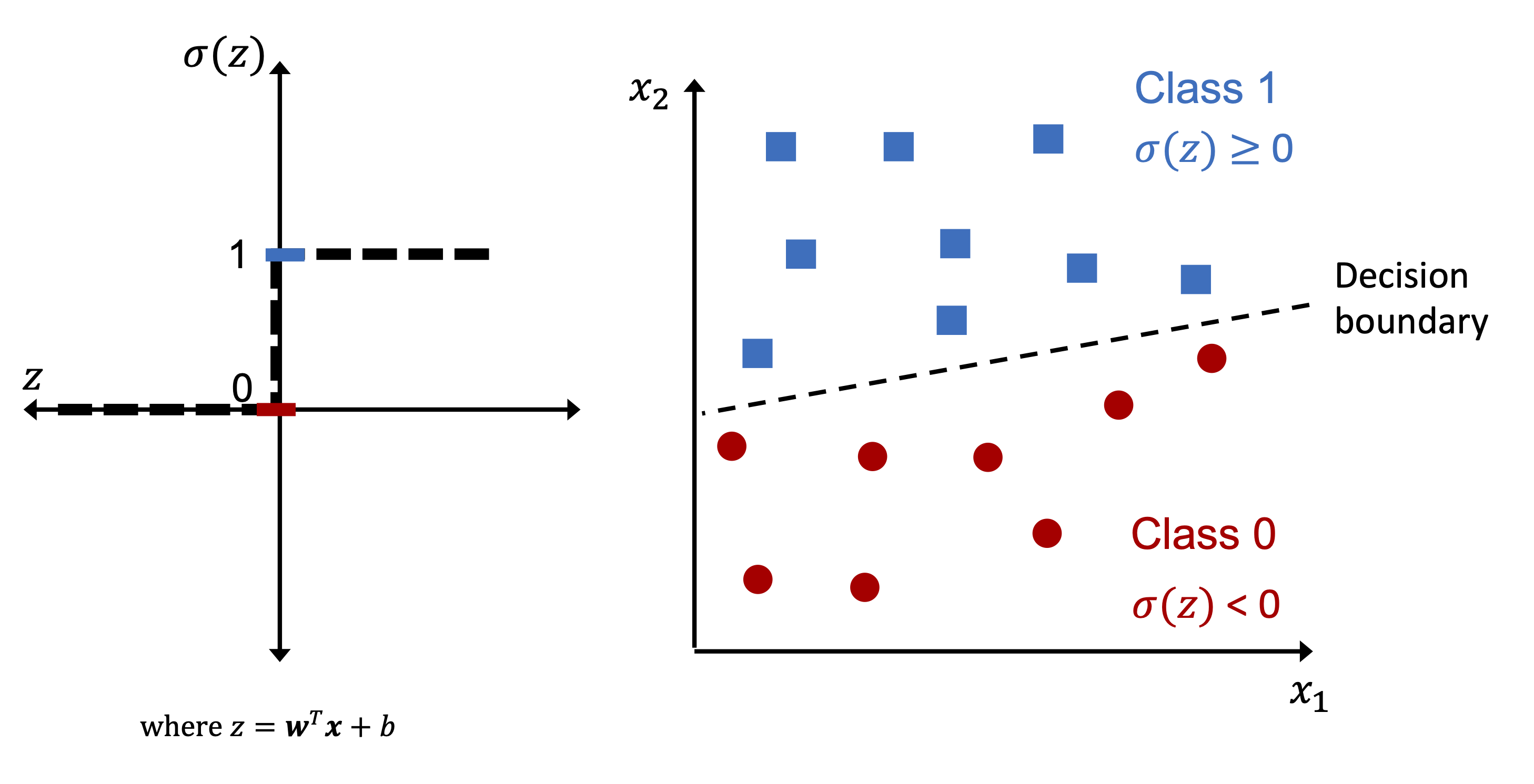 

import numpy as np
import pandas as pd
from sklearn.datasets import load_iris

iris = load_iris()
df = pd.DataFrame(data= np.c_[iris['data'], iris['target']],
                  columns= iris['feature_names'] + ['target'])

X = df.iloc[:100,[0,2]].values
y = df.iloc[0:100,4].values
y = np.where(y == 0, -1, 1)

import matplotlib.pyplot as plt

plt.scatter(X[:50,0],X[:50,1],color='red', marker='o',label='setosa')
plt.scatter(X[50:100,0],X[50:100,1],color='blue', marker='x',label='versicolor')
plt.xlabel('sepal length (cm)')
plt.ylabel('petal length (cm)')
plt.legend(loc='upper left')
plt.show()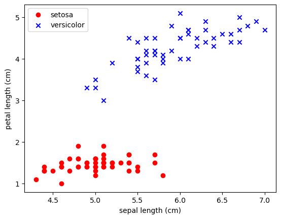

childe = Perceptron()
childe.fit()

# eta parameter - how fast you will learn
childe.eta

# how many mistakes 

childe.errors_ 

# weights are solution
childe.w_
# in our case we have two weights

class Perceptron():
    def __init__(self, n_iter=10, eta=0.01):
        self.n_iter = n_iter
        self.eta = eta
        
    def fit(self, X, y):
        self.w_ = np.zeros(1+X.shape[1])
        self.errors_ = []
        for _ in range(self.n_iter):
            pass
        return self

import random

class Perceptron():
    
    def __init__(self, eta=0.01, n_iter=10):
        self.eta = eta
        self.n_iter = n_iter
    
    def fit(self, X, y):
        
        #self.w_ = np.zeros(1+X.shape[1])
        self.w_ = [random.uniform(-1.0, 1.0) for _ in range(1+X.shape[1])] 
        self.errors_ = []
        
        for _ in range(self.n_iter):
            errors = 0
            for xi, target in zip(X,y):
                #print(xi, target)
                update = self.eta*(target-self.predict(xi))
                #print(update)
                self.w_[1:] += update*xi
                self.w_[0] += update
                #print(self.w_)
                errors += int(update != 0.0)
            self.errors_.append(errors)
        return self
    
    def net_input(self, X):
        return np.dot(X, self.w_[1:])+self.w_[0]
    
    def predict(self, X):
        return np.where(self.net_input(X)>=0.0, 1, -1)

# like in scikitlearn
ppn = Perceptron()
ppn.fit(X,y)

<__main__.Perceptron at 0xffff71056350>

print(ppn.errors_)
print(ppn.w_)

[1, 0, 0, 0, 0, 0, 0, 0, 0, 0]
[-0.514977988012733, -0.31227988722357647, 0.7705418793848033]

ppn.predict(np.array([-3, 5]))

array(1)

import pickle
with open('model.pkl', "wb") as picklefile:
    pickle.dump(ppn, picklefile)

# dodatkowa funkcja

from matplotlib.colors import ListedColormap

def plot_decision_regions(X,y,classifier, resolution=0.02):
    markers = ('s','x','o','^','v')
    colors = ('red','blue','lightgreen','gray','cyan')
    cmap = ListedColormap(colors[:len(np.unique(y))])

    x1_min, x1_max = X[:,0].min() - 1, X[:,0].max()+1
    x2_min, x2_max = X[:,1].min() -1, X[:,1].max()+1
    xx1, xx2 = np.meshgrid(np.arange(x1_min, x1_max, resolution),
                           np.arange(x2_min, x2_max, resolution))
    Z = classifier.predict(np.array([xx1.ravel(), xx2.ravel()]).T)
    Z = Z.reshape(xx1.shape)
    plt.contourf(xx1, xx2, Z, alpha=0.4, cmap=cmap)
    plt.xlim(xx1.min(), xx1.max())
    plt.ylim(xx2.min(),xx2.max())

    for idx, cl in enumerate(np.unique(y)):
        plt.scatter(x=X[y == cl,0], y=X[y==cl,1], alpha=0.8, c=cmap(idx), marker=markers[idx], label=cl)

# dla kwiatków

plot_decision_regions(X,y,classifier=ppn)
plt.xlabel("dlugosc dzialki [cm]")
plt.ylabel("dlugosc platka [cm]")
plt.legend(loc='upper left')
plt.show()

/tmp/ipykernel_37211/2939353802.py:21: UserWarning: *c* argument looks like a single numeric RGB or RGBA sequence, which should be avoided as value-mapping will have precedence in case its length matches with *x* & *y*.  Please use the *color* keyword-argument or provide a 2D array with a single row if you intend to specify the same RGB or RGBA value for all points.
  plt.scatter(x=X[y == cl,0], y=X[y==cl,1], alpha=0.8, c=cmap(idx), marker=markers[idx], label=cl)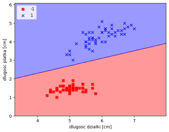

Image(filename='./img/02_09.png', width=600)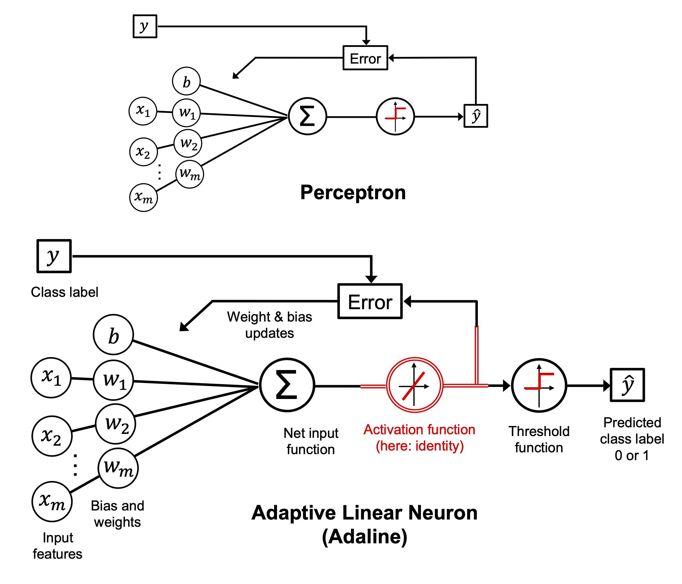 

# ZADANIE - Opisz czym różni się poniższy algorytm od Perceprtona ? 
class Adaline():
    '''Klasyfikator  - ADAptacyjny LIniowy NEuron'''
    def __init__(self, eta=0.01, n_iter=10):
        self.eta = eta
        self.n_iter = n_iter

    def fit(self, X,y):
        import random
        self.w_ = [random.uniform(-1.0, 1.0) for _ in range(1+X.shape[1])]
        self.cost_ = []

        for i in range(self.n_iter):
            net_input = self.net_input(X)
            output = self.activation(X)
            errors = (y-output)
            self.w_[1:] += self.eta * X.T.dot(errors)
            self.w_[0] += self.eta * errors.sum()
            cost = (errors**2).sum() / 2.0
            self.cost_.append(cost)
        return self

    def net_input(self, X):
        return np.dot(X, self.w_[1:]) + self.w_[0]

    def activation(self, X):
        return self.net_input(X)

    def predict(self, X):
        return np.where(self.activation(X) >= 0.0, 1, -1) 

ad = Adaline(n_iter=20, eta=0.01)

ad.fit(X,y)

print(ad.w_)

plot_decision_regions(X,y,classifier=ad)
# plt.xlabel("dlugosc dzialki [cm]")
# plt.ylabel("dlugosc platka [cm]")
plt.legend(loc='upper left')
plt.show()

[-1.1586984096359621e+31, -6.471276925359209e+31, -3.6205813799954466e+31]

/tmp/ipykernel_37211/2939353802.py:21: UserWarning: *c* argument looks like a single numeric RGB or RGBA sequence, which should be avoided as value-mapping will have precedence in case its length matches with *x* & *y*.  Please use the *color* keyword-argument or provide a 2D array with a single row if you intend to specify the same RGB or RGBA value for all points.
  plt.scatter(x=X[y == cl,0], y=X[y==cl,1], alpha=0.8, c=cmap(idx), marker=markers[idx], label=cl)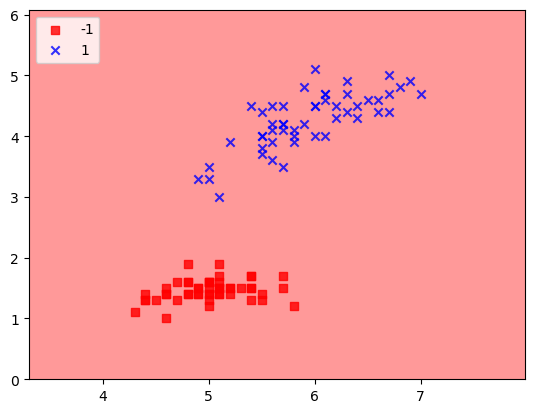

ad.cost_[:10]

[1704.8690320472695,
 2446158.759682741,
 3815654556.186715,
 5951879816203.038,
 9284088181450494.0,
 1.4481860525196487e+19,
 2.25896480270697e+22,
 3.5236646361774773e+25,
 5.496416966465838e+28,
 8.57363074768274e+31]

ad2 = Adaline(n_iter=100, eta=0.0001)

ad2.fit(X,y)

plot_decision_regions(X,y,classifier=ad2)
# plt.xlabel("dlugosc dzialki [cm]")
# plt.ylabel("dlugosc platka [cm]")
plt.legend(loc='upper left')
plt.show()

/tmp/ipykernel_37211/2939353802.py:21: UserWarning: *c* argument looks like a single numeric RGB or RGBA sequence, which should be avoided as value-mapping will have precedence in case its length matches with *x* & *y*.  Please use the *color* keyword-argument or provide a 2D array with a single row if you intend to specify the same RGB or RGBA value for all points.
  plt.scatter(x=X[y == cl,0], y=X[y==cl,1], alpha=0.8, c=cmap(idx), marker=markers[idx], label=cl)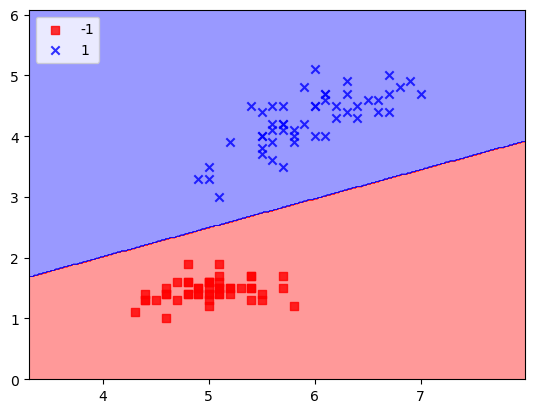

print(ad2.w_)

ad2.cost_[-10:]

[-0.05106024193782033, -0.2323920213934253, 0.4867801970114242]

[12.14492536723885,
 11.934276461271914,
 11.728250635884299,
 11.526746421759194,
 11.329664576671968,
 11.136908036608968,
 10.94838186795925,
 10.763993220755546,
 10.583651282941581,
 10.40726723564312]

%%file app.py

import pickle
import numpy as np
from flask import Flask, request, jsonify

class Perceptron():
    
    def __init__(self, eta=0.01, n_iter=10):
        self.eta = eta
        self.n_iter = n_iter
    
    def fit(self, X, y):
        self.w_ = [random.uniform(-1.0, 1.0) for _ in range(1+X.shape[1])] 
        self.errors_ = []
        
        for _ in range(self.n_iter):
            errors = 0
            for xi, target in zip(X,y):
                update = self.eta*(target-self.predict(xi))
                self.w_[1:] += update*xi
                self.w_[0] += update
                errors += int(update != 0.0)
            self.errors_.append(errors)
        return self
    
    def net_input(self, X):
        return np.dot(X, self.w_[1:])+self.w_[0]
    
    def predict(self, X):
        return np.where(self.net_input(X)>=0.0, 1, -1)

# Create a flask
app = Flask(__name__)

# Create an API end point
@app.route('/predict_get', methods=['GET'])
def get_prediction():
    # sepal length
    sepal_length = float(request.args.get('sl'))
    petal_length = float(request.args.get('pl'))
    
    features = [sepal_length, petal_length]

    # Load pickled model file
    with open('model.pkl',"rb") as picklefile:
        model = pickle.load(picklefile)
        
    # Predict the class using the model
    predicted_class = int(model.predict(features))
    
    # Return a json object containing the features and prediction
    return jsonify(features=features, predicted_class=predicted_class)

@app.route('/predict_post', methods=['POST'])
def post_predict():
    data = request.get_json(force=True)
    # sepal length
    sepal_length = float(data.get('sl'))
    petal_length = float(data.get('pl'))
    
    features = [sepal_length, petal_length]

    # Load pickled model file
    with open('model.pkl',"rb") as picklefile:
        model = pickle.load(picklefile)
        
    # Predict the class using the model
    predicted_class = int(model.predict(features))
    output = dict(features=features, predicted_class=predicted_class)
    # Return a json object containing the features and prediction
    return jsonify(output)


if __name__ == '__main__':
    app.run(host='0.0.0.0', port=5000)

Overwriting app.py

import requests
response = requests.get("http://127.0.0.1:5000/predict_get?sl=6.3&pl=2.6")
print(response.content)

b'{"features":[6.3,2.6],"predicted_class":-1}\n'

import requests
json = {"sl":2.4, "pl":2.6}
response = requests.post("http://127.0.0.1:5000/predict_post", json=json)
print(response.content)

b'{"features":[2.4,2.6],"predicted_class":1}\n'